Simulation

This section explains the settings to run the windshield defrost simulation. Initially, flow field simulation is performed to develop flow field. Then, transient heat transfer simulation is performed for defrost analysis.

Flow field simulation

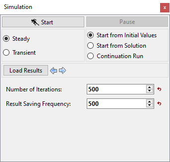
Click Simulation Panel.
Define Number of Iterations as 500 and Result Saving Frequency as 500 respectively.
After you save the project, click Start to run the simulation (see, Figure 7.283).
The result files are saved as filename.sres in the working folder (Example: "windshield_defrost_flow_model.sres").

The residuals for the steady state simulation are displayed under the Residual Tab in the Plot Panel as shown in Figure 7.284.

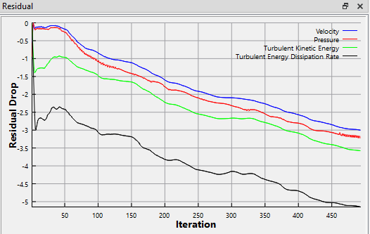
Figure 7.283 - Steady simulation settings

Figure 7.284 - Residual-Steady

´	Note: The default Converge Criterion is 0.001 for steady state simulations. A steady state simulation runs until the residual for each variable drops by 3 orders or until the maximum Number of Iterations is reached, at which time a results file will be saved as: “filename.sres.

Heat transfer Simulation settings

Once steady state simulation is completed, setup for defrost (solidification and melting) conjugate heat transfer simulation and use the flow field developed by the steady state simulation and restart transient simulation.

Click Select Modules in the Model Panel. The Physical Model Selection dialog box opens.
Select Heat under Available Modules list, click Add.
Click Close to close the Physical Model Selection dialog box.
Uncheck Flow and Turbulence in the Model Panel.

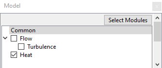
Figure 7.285 - Adding Heat modules

Inlet

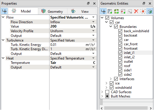
Select inlet_i1 from the Boundaries list under Volumes in the Geometric Entities Panel.
Enter Tair C for Temperature under Heat list.

Figure 7.286 - Inlet Condition

Initial Condition

Select car Volume in the Geometric Entities Panel.
Select Model Tab in the Properties Panel and enter 1.1766 kg/m³ for Density under Common drop-down list.
Enter -4 C for Initial Condition Value under Heat drop-down list.

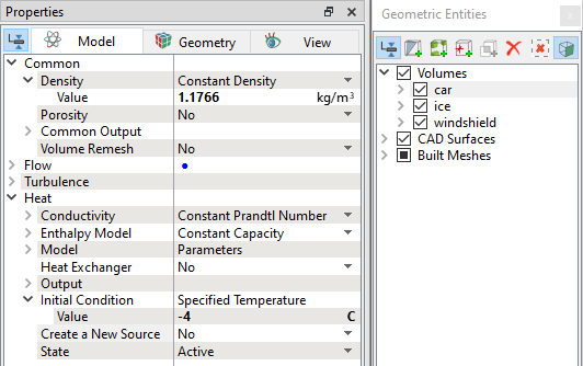
Figure 7.287 - Initial Condition

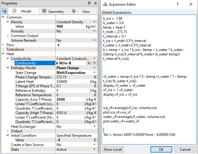
Ice Heat Transfer Properties

Select ice Volume in the Geometric Entities Panel.
Select Model Tab in the Properties Panel.
Select Constant Conductivity under Conductivity drop-down of Heat list.
Click Edit Expression icon in the Conductivity under Heat list, to open the Expression Editor dialog box .
Copy and paste the expressions written under Description drop-down list for Global Expressions editor of Simerics-MP+ as shown in Figure 7.288.
Description
k_ice = 1.88
k_water = 0.6
temp = heat.T
t_melt = 273.15
t_interval = 0.1
t_ice = t_melt-0.5*t_interval
t_water = t_melt+0.5*t_interval
k = temp < t_ice ? k_ice : (temp > t_water ? k_water : ((temp-t_ice)/t_interval*k_water+(t_water-temp)/t_interval*k_ice))

vf_water = temp<t_ice ? 0 : (temp>t_water ? 1 : (temp-t_ice)/(t_water-t_ice))
display.vf_water = vf_water
vf_ice = 1-vf_water
display.vf_ice = vf_ice

ice_vf=average(vf_ice, volume.ice)
plot.ice_vf=ice_vf
water_vf=average(vf_water, volume.ice)
plot.water_vf=water_vf

Tair = (time<2400? 0.04500*time - 4.00000:104)
Click OK, to close the Expression Editor dialog box.
Enter k W/m-K for Conductivity.
Select Phase Change under Enthalpy Model drop-down list.
Select Melt/Evaporation under State Change drop-down list.
Enter 2040 J/kgK for Capacity (Low T Phase).
Enter -4 C for Value under Initial Condition.

Figure 7.288 - Ice Heat transfer Condition

Windshield Properties

Select windshield Volume in the Geometric Entities Panel.
Select Model Tab in the Properties Panel.
Select Constant Conductivity under Conductivity drop-down of Heat list.
Enter 0.9 W/m-K for Conductivity.
Select Constant Capacity under Enthalpy Model drop-down list.
Enter 900 J/kgK for Capacity.
Enter -4 C for Value under Initial Condition.

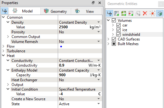
Figure 7.289 - Windshield properties

Transient Simulation Settings

Click Simulation Panel.
Select Transient.
Select Load Results and load the steady state results defrost_car_flow_model.sres.
Enter Simulation Time (Duration) and Number of Time Steps to 2400 s and 1200 respectively.
Define Number of Iterations and Result Saving Frequency as 25 and 60 respectively (see, Figure 7.290).
After you save the project, click Start to run the simulation. Make sure you are restarting the transient simulation with steady state results.
The result files are saved as filename_060.sres in the working folder.

Note: The Result Saving Frequency option in the Simulation Panel is set to a small value (say 5 or 10) before running the simulation to obtain better animations.

The residuals are displayed under the Residual Tab in the Plot Panel (see, Figure 7.291).

Figure 7.290 - Transient Simulation settings

Figure 7.291 - Residuals - Transient simulation

Note: The default Converge Criterion is 0.1 for Transient simulations. When the residuals for all the variables drop by one order or the maximum Number of Iterations is reached, the calculation proceeds to the next time-step.