14.1 Theory
This section explains the discretization of the governing equations, linearization and solving the linear system of equations.
Discretization and Solution
To illustrate the finite volume methodology, the general form of the transport equation of a passive scalar,  is considered as follows:

|
where from left to right, the terms represent the transient, advection (convection), diffusion and source terms of the transporting scalar- respectively.
Using the Finite Volume Method (FVM), equation 14.1 is first integrated over an arbitrary volume,  . Applying the Green-Gauss theorem, the volume integrals of the convection and diffusion terms are converted to surface integrals. In a moving reference frame with the mesh velocity
  ,the integral form of the conservation equation for scalar-
 is then expressed as:

|
where

|
General scalar representing any dependent variable |

|
Velocity vector  |

|
Mesh velocity. It is zero if there is no geometry change or mesh movement |

|
External/User source for scalar- |

|
Effective diffusion coefficient of scalar- |

|
Control volume, which is a function of time in moving meshes |

|
Surface area (magnitude) of the control volume  , commonly referred to as “face" , commonly referred to as “face" |

|
Normal vector of the control volume surfaces |

|
Volume integral |

|
Surface integral. In equation 14.2, the Green-Gauss Theorem is applied to convert the volume integrals of the convection and diffusion terms to surface integrals. |
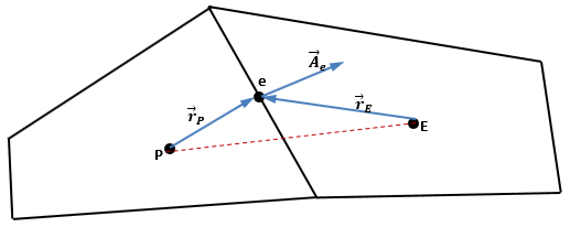
equation 14.2 is applied to each individual control volume cell in the computational domain. As indicated by the 2D sketch in Figure 14.1, over an arbitrary control volume " ",
",  is stored at the cell center (point P) and is assumed to remain unchanged within the cell. To discretize equation 14.2 over "
 ", the volume integrals (transient and source terms) are calculated using the cell center values, while the surface integrals (the advection and diffusion) are approximated by the sum of the face values across all the surfaces enclosing the control volume "
 ". After discretization, the resulting equation has the form:

|
where

|
Transient term. It is determined by temporal schemes |

|
Mass flux through surface/face “ ”: ”:  |

|
Area vector of surface “ ”: ”:  |

|
Gradient of  at the surface “ at the surface “ ” ” |

|
Effective diffusion coefficient at the surface “ ”; ”; |

|
Control volume surface between cell “ ” and “ ” and “ ” (face “ ” (face “ ”) ”) |

|
Number of surfaces enclosing the cell |
The individual terms of equation 14.3 should be discretized and linearized. This is accomplished by:
- Spatial discretization of the diffusion and advection terms. Since Simerics-MP solves and then stores the discrete values of
 at (
at ( and
and  in Figure 14.1), the values at cell faces
  must be calculated from the cell values.
 - Temporal discretization for approximation of the transient terms in unsteady flows.
- Linearization of the source term.
The spatial and temporal discretization are implemented using various numerical schemes, which have different orders of numerical accuracy. More detailed descriptions on the numerical schemes are given in the following subsections.
Spatial Discretization Schemes
Advection Terms
The advection term in equation 14.3 requires the face value  to be approximated in terms of the cell values
  and gradients
  . The advection schemes implemented in Simerics-MP can be written in a general form:

|
With the use of different values for parameters  the following commonly-used advection schemes can be easily derived:
First -Order Upwind (or Upwind) scheme

|
2nd Order Upwind scheme

|
Central Difference Scheme

|
Blended Higher Order Scheme
It is well known that the first-order upwind scheme is unconditionally stable but could be too diffusive. The second-order upwind and the central-differencing schemes have a higher order of accuracy, but can produce unbounded solutions and non-physical wiggles, which in turn can lead to stability problems for the numerical procedure. These stability problems can often be avoided by blending either of them with the first-order upwind scheme as follows:

|
where  is the blend factor.
Diffusion Terms
The diffusion terms in equation 14.3 are approximated using the central-difference scheme so they always have the second-order accuracy. On the face- , the diffusion coefficient
  is usually obtained from weighted average or harmonic average of the cell center values at the control volume "
 " and "
 ". The surface normal gradient is decomposed into two terms: the gradient/change directly between the two cells, and the secondary gradient along the face-"
 ":
":

|
where

|
Discretized values of  at the control volume cells " at the control volume cells " " and " " and " ". ". |

|
Reconstruction gradients of  at the control volume cells " at the control volume cells " " and " " and " ". ". |
In equation 14.9, the first term is considered as the diffusion term, while the secondary gradient term, originated from the non-orthogonal mesh, is treated as source terms in the final linear equation of the discretized  .
.
Source Term Linearization
The term  represents the net/total source terms for scalar-
 , which may contain contributions from different physical mechanisms/ models. For example, in momentum equations,
  can be sources from pressure gradients, body forces, and/or momentum sink in porous media. They often present large sources and must be linearized properly to ensure numerical stability.
Though some of the sources terms, such as the pressure gradients in momentum equations are discretized using surface integral over all the faces enclosing a control volume cell, most of the sources terms are generally discretized over a control volume. In equation 14.3,  is linearized in the following general form to improve the robustness in the iterative numerical procedure:

|
where  always has non-negative values,
  .
.
Temporal Discretization Schemes
For transient flow simulations, the governing equations must be discretized in both space and time, as shown in equation 14.3. At a given time, the spatial discretization over a control volume is the same as in the steady-state simulations, while the temporal discretization involves the integration of all the terms in the governing equations over the time interval  . In Simerics-MP, different temporal schemes are implemented to approximate the transient term,
  .
.
To describe the temporal discretization schemes, for clarity, the time-dependent, partial differential transport equation 14.1 may be rewritten in a simple form under the constants of  and
and  as:
as:

|
Assuming that  ,
,  and
and  are the numbers of the time-step at the physical time
  ,
,  and
and  respectively, and
  ,
,  and
and  are the corresponding values of scalar-
 , we have the following expression over the time interval
  :
:

|
where the function  , may represent the spatial discretization, consisting of the terms of convection, diffusions, external sources and/or momentum sinks in the flow governing equations. In the temporal discretization,
  can be estimated by
  ,
,  or a blend of
  and
and  respectively.
The integration of the transient term  is straightforward. Introducing two sub-time steps,
  and
and  at the time intervals
  and
and  respectively, we can estimate the values of
  as:
as:

|
|

|
Then the term  can be discretized as:

|
where  and
and  are interpolation coefficients. Assuming that

|
and substituting equations equation 14.13, equation 14.14 ,equation 14.16 into equation 14.15 and rearranging the terms, we have the following general expression:

|
With equation 14.17 and the estimated value of  the discretization of equation 14.12 results in the following widely used time integration schemes:
Euler Explicit Method (Forward Scheme)
Setting  in equation 14.17 and
  , the equation 14.17 becomes the first-order Euler explicit time scheme:

|
In this forward/time-marching method, the evaluation of  is entirely based upon the known values at the previous time-step. This scheme is simple and non-iterative, but it can be numerically unstable, especially for stiff equations with larger time steps. Therefore, for both accuracy and stability, the required time-step
  is usually very small. As a result, the Euler Explicit Method is rarely used when solving the highly non-linear Navier-Stokes equations in the finite volume method.
Euler Implicit Method (Backward Scheme)
To improve the accuracy and numerical robustness, the Euler implicit time scheme is almost always used in CFD simulations:

|
The implicit time scheme is more complicated and must be solved iteratively since  is approximated using the unknown
  . However, the implicit method allows much larger time-step than the explicit scheme due to its robustness and can also offer high-order time accuracy. For example, with different
  values, equation 14.19 returns the following commonly used time schemes:
 , First order implicit time scheme
 , Three-level second-order implicit time scheme.
It may be noted that in the implicit time integration, the first-order time scheme is numerically stable and physically bounded unconditionally. The three-level second-order time scheme could return physically unbounded solutions (unde-and/or-overshoot) where there are larger gradients or sharp fronts of a transient solution. With a proper  between 0 and 1, a blended formulation of the first-order and second-order time schemes can achieve bounded solution while mostly maintaining second-order time accuracy. In this sense the factor
  is also called the blending factor. In Simerics-MP,
  is a user input parameter, by default it is set to 0.1. Three-level second-order implicit time scheme is the Simerics-MP recommended method to achieve higher accuracy in time when first order implicit method is inadequate.
Crank-Nicolson Method
The Crank–Nicolson method is based on the trapezoidal rule when integrating  in equation 14.12. It is an implicit time scheme with the second-order time accuracy. In the mathematical form, this method is a combination of the first order forward Euler method and the backward Euler method:

|
By default, the factor  . Compared to the three-level second-order implicit time scheme in equation 14.19, the Crank-Nicolson method only requires the values at two-time levels
  and could obtain oscillatory solutions for some cases. When it happens a higher
  value, for example 0.6 should be used to eliminate the oscillation.
Transient Terms in Transport equation
With the described temporal discretization method, the transient term in equation 14.3 can be easily approximated using one of the implicit time schemes. To conform with the conventional notation, we first use  to represent the value at the present time-step, and the old values at the two previous time steps. Then after rearranging equation 14.17, the general formulation of the implicit time scheme is rewritten as:

|
With the application of equation 14.21, the transient term in equation 14.3 can be expressed as:

|
Solving the Linear Systems-Solution matrix
With the temporal and spatial schemes, the discretized transport equation 14.3 contains the unknown scalar variable  at the center of the control volume cell as well as the unknown values in the surrounding neighbor cells. This equation is, in general, nonlinear with respect to the solved variable
  . However, with the inclusion of
  -dependent terms in the coefficients, the final discretized governing equation can be written in a linear from:

|
where " " represents the neighboring cells of an arbitrary control volume cell, whose total number depends on the mesh topology, but is typically equal to the number of faces enclosing the cell.
Similar equations can be obtained over every control volume in a computational domain. Together, they result in a set of algebraic equations with a sparse coefficient matrix. For scalar equations, Simerics-MP solves this linear system of equations using either an Algebraic Multi-Grid-AMG Solver or Conjugate Gradient Squared-CGS Linear Solver. The solution accuracy for equation 14.23 is determined by the given tolerance or the maximum number of sweeps within the linear solvers.
Since the values of  ,
,  and
and  in equation 14.23 over each control volume cell are the functions of the solved variable
  , an iterative solution algorithm, in which
  ,
,  and
and  are updated and the equation 14.23 is solved repeatedly in a loop, must be applied to obtain the numerical solution of
  .
.
In Simerics-MP, this linear system of equations is solved in  -form iteratively, in which the variable
  is assumed to be equal to the old/ estimated value,
  and a correction
  as:
as:

|
where  is zero when the solution is fully converged.
Diagonal Relaxation
Furthermore, to enhance the diagonal dominance of the linear system, a diagonal relaxation factor  , is introduced into equation 14.23:

|
where  has a non-negative value. Since it is applied to the discretized equation,
  is also called as the implicit relaxation factor.
From equation 14.24 - equation 14.25, the solved variable, the correction  , is thus as follows:

|
To ensure numerical stability during the iterative process, an explicit relaxation factor,  can also directly applied for the computation of
  using the solved
  :
:

|
where  is between 0 and 1. By default,
  .
.
Linear Solver Tolerance and Sweeps
The iterative solution can be controlled by using a desired convergence tolerance called the Linear Solver Tolerance and/or the number of Sweeps.
- When the correction of a given variable drops below its Linear Solver Tolerance, the solver will end the current calculation loop of the variable.
- Sweeps denote the number of iterative cycles to be performed to obtain the numerical solution of
 .
.
When the Linear Solver Tolerance or the maximum number of Sweeps is reached the solver will also end the current calculation loop for the variable and proceed to the next calculation. The solution accuracy for equation 14.23 is therefore determined by the given tolerance or the maximum number of sweeps within the linear solvers.
Pressure-Based Flow Solver
In Simerics-MP, the pressure-based finite-volume approach is adopted for solving the conservation of mass and momentum for all fluid flows. In this method, the velocity field is obtained directly from the discretized momentum equations. The pressure field is obtained by solving a pressure correction equation, which is derived from the discretized continuity and the momentum equations in a way that the velocity field, corrected by the pressure, satisfies the continuity.
Discretization of Governing Equations
As for the scalar transport equation, described in Discretization and Solution, the flow governing equations of continuity and momentum can be discretized following the same approach:
Continuity: For the mass conversation, the continuity equation solved has the general integral form:

|
Over an arbitrary control volume cell, the discretized equation has the following expression:

|
Momentum of Uj: With the introduction of  to represent the Cartesian velocity component
  ,
, and
and  respectively, the conservation equation of
  -momentum can be written as:

|
Integrating equation 14.30 over the control volume, the final discretized momentum equation upon applying the mass continuity equation 14.29 and mathematical rearrangement, can be written as:

|
where

|
The diagonal coefficient excluding the transient contribution:  |

|
Link coefficients including diffusion and upwind advection terms |

|
Face pressure |

|
Component- in unit vector in unit vector  |

|
Body force acting upon  |

|
Sources consisting both physical and numerical terms.
|
 , first order implicit time scheme.
 , second order implicit time scheme
In equation 14.31, the face pressure  is estimated from the cell-center pressure values obtained from solving the pressure correction equation:

|
where

|
Linear pressure scheme |

|
Second-order pressure scheme |
As described for the general scalar equation 14.23, the discretized momentum equations are also solved in the  -form. For the corrections of the three velocity components
  , the solved equation has the general form:

|
And the velocity component  has the value:

|
where  is the diagonal relaxation factor for velocity, which has the default value of 0.3; and
  is the explicit velocity relaxation factor having zero as the default value.
Pressure-Velocity Coupling
To close the discretized momentum equation 14.31, the face fluxes  and the cell-center flow pressure in equation 14.32, need to be calculated. For collocated, pressure-based finite volume solvers, the face fluxes are computed following the Rhie and Chow approach, while the pressure is obtained using the SIMPLE (Semi-Implicit Method for Pressure Linked Equations) algorithm and its variants. Based on the sketch in Figure 14.1, the algorithms of pressure-velocity coupling adopted in Simerics-MP is briefly described in this section.
Flux Formulation
As indicated in the discretized scalar equation 14.3, at the face “ ” between the two control volumes “
 ” and “
 ”, the face mass flux has the expression:

|
where  is face density, which is also estimated using the cell-center values. For variable density flows, different interpolation schemes (upwind, 2nd-order upwind and central difference) can be applied, though by default, it is set to the first-order upwind density scheme.
In addition, the term  , is the face grid flux. With a given mesh velocity, it can be easily calculated. Therefore, the only term in equation 14.35 that needs to be computed is the face volumetric flux:

|
In Simerics-MP the face velocity components,  are computed following the Rhie and Chow method. For brevity, only the component
  is derived in detail. From equation 14.31, the discretized
  -momentum equation can be rewritten as:

|
where  is the number of faces enclosing the control volume “
 ”, and the other terms are defined as:

|
|

|
|

|
|

|
Similarly, for the control volume cell “ ” and the face “
 ”, we can have the discretized
  -momentum equations in the following expressions:

|
|

|
Following the approach proposed by Rhie and Chow1Rhie CM and Chow WL (1983), Numerical Study of the Turbulent Flow past an Airfoil with Trailing Edge Separation, AIAA J., Vol.21. and including a weighting function  (with the default value of 0.5), we can assume that:

|
|

|
Substituting equation 14.37-equation 14.44 into equation 14.45, we have the face velocity of the  -component,
  , as:
, as:

|
14.46 |
Similarly, the face velocity components  and
and  can be evaluated from the discretized
  -momentum and
  -momentum equations respectively. Substituting them into the equation 14.36, the face volumetric flux,
  and then the face mass flux
  in equation 14.35 are computed.
Pressure Correction Equation
Once the face flux is computed, the construction of the pressure correction equation is straightforward. Introducing correction terms for the relevant quantities/variables, we can express their new values as the sum of the old values and the corresponding correction terms as:

|
where  represent the old values obtained from the previous iteration or time-step.
Substituting equation 14.47 into the discretized continuity equation 14.29, we have the correction equation after rearrangement:

|
Note that the term on the right-hand side is the mass imbalance over the control volume. With the correct flow field (a fully converged solution), it is zero so that the local continuity is satisfied.
Following the SIMPLE type of algorithms (Simple, SimpleC and SimpleS), the relations between the velocity correction and pressure correction are estimated based on the discretized momentum equations. For example, we can rewrite equation 14.43 as:

|
Assuming the following

|
Then we have

|
where the coefficient,  depends on the SIMPLE type schemes, or the assumption in equation 14.49.
In the same fashion,  and
and  are estimated. Substituting them into equation 14.48, the final pressure-correction equation is:

|
where  is the diagonal relaxation factor for pressure correction.
With the value of  obtained by solving equation 14.51, the pressure field is computed as

|
where  is between 0 and 1. By default,
  . As for the auto relaxation factor
  , adds linear relaxation automatically for the pressure solution based on mesh quality in Simerics-MP.
The pressure correction,  has also been used to correct the cell center velocity components, face velocity/mass fluxes and other flow variables to satisfy the continuity and enhance numerical stability.
Pressure-Based Segregated Algorithm
As described for the scalar equation 14.23, the discretized momentum and pressure-correction equation 14.31 and equation 14.51 are strongly non-linear and tightly coupled together since the coefficients and source terms are functions of the solved variables. As a result, an iterative solution algorithm such as, the widely-used pressure-based segregated solver, must be adopted to obtain a converged numerical solution.
In Simerics-MP, while the three velocity components  are solved in a coupled manner, while the pressure correction equation is solved separately. The solver can be run in both steady-state and transient modes. For a steady-state simulation, the solution process consists of a number of iterations, and within each iteration, the governing equations are solved in the order of momentum, pressure/pressure-correction and additional scalars when appropriate. The simulation stops when the solution is fully converged with a given convergence criteria or when the number of iterations reaches the pre-determined limit. In the transient mode, the implicit temporal method or iterative time-advancement scheme is employed. For a given time-step, the iterative scheme is the same as the steady-state solver-all the equations are solved iteratively until the convergence criteria are met. The simulation then advances to the next time-step. The solution procedure may be illustrated in Figure 14.2. Note that though it is for the iterative time advancement solution, it also applies for the steady-state run when the outermost loop for the time advancement is ignored.
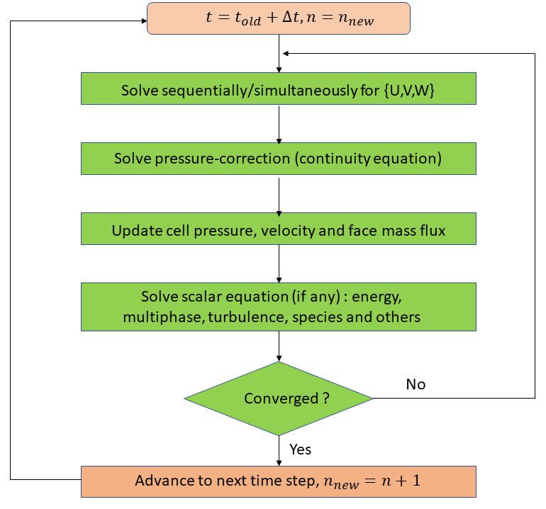
Figure 14.2 - Overview of the pressure based solution method