9 - Optimization Module and Tutorial
Optimization module in Simerics-MP+ allows to perform geometry optimization in the same GUI. This module utilizes the Bayesian Inference method for optimization and Latin Hypercube Sampling for Design of Experiments (DOE). The module has the options to utilize the Simerics Volume Remesh capability or a third-party parametric geometry modeler through a dedicated interface to perform geometry optimization.
|
To activate the Optimization module:
- Click Select Modules in the Model Panel. The Physical Model Selection dialog box opens Figure 9.1.
- Select Controller module under Available Modules and click Add.
|
|
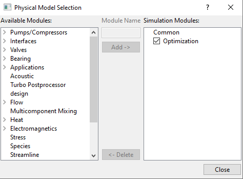
Figure 9.1 - Optimization module
|
Structure of optimization is divided into three categories. Each section contains set of parameters, which must be defined.
Sampling Method
The two options available under Sampling Method, as shown in Figure 9.3 are Random or From Result.
|
|
|
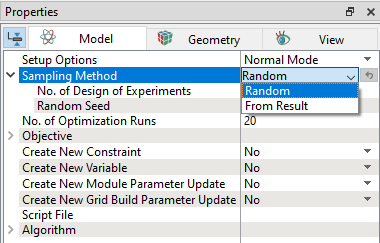
Figure 9.2 - Sampling Method
|
Optimization Setup
The list of options available under Objective are explained below.
- Objective: The two options available under Objective, as shown in Figure 9.3 are Maximize or Minimize.
- Expression: This allows to specify the objective function.
- Processing method: This allows to choose the processing method of the objective function, such as
- Last Value: The last value of the objective function in simulation.
- Mean Value: The averaged value of the objective function over the last (Number of Values) time steps/iterations.
- Standard Deviation: The square root of the average of the deviations of objective function over the last (Number of Values) time steps/iterations, from the mean value.
|
|
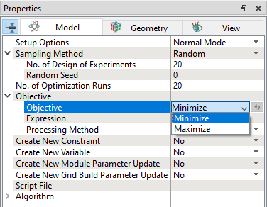
Figure 9.3 - Objective
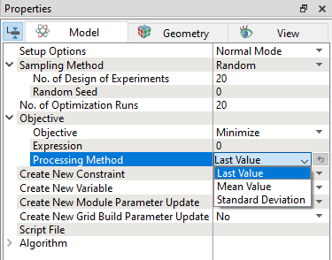
Figure 9.4 - Processing method
|
- Constraint: Select Add a Constraint from Create New Constraint dropdown to create new Constraints. On creating new Constraint, few more options are available.
- Expression: The constraint function can be specified here.
- Processing method:
- Limit: The limit of the constraints can be specified here.
|
|
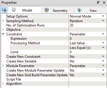
Figure 9.5 - Constraints
|
- Variable: Select Add a Variable from Create New Variable dropdown to create new Variables. On creating new Variable, few more options are available.
- Variable Name: The user-defined name of the variable. This name can be referred in expression editor.
- Minimum: The lower bound of the variable range.
- Maximum: The upper bound of the variable range.
|
|
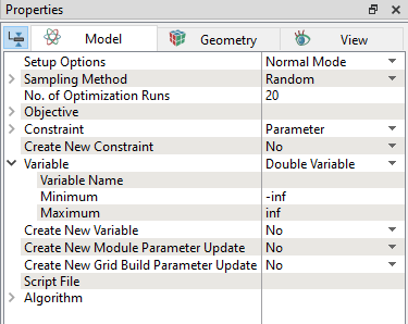
Figure 9.6 - Variables
|
- Module Parameter Update: Select Add a parameter update from Create New Module Parameter Update dropdown to create new Module Parameter. On creating new Module Parameter, few more parameters are available.
- Simulation Module: Allows to choose the module selected as part of current simulation.
- Parameter Name: Allows to choose parameters related to that module from the dropdown. On selecting parameter, User Expressions option appears. User can enter expressions controlling the parameter selected.
|
|
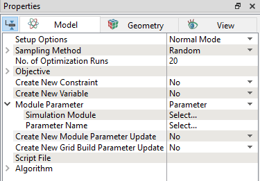
Figure 9.7 - Module Parameter
|
- Grid Build Parameter Update: Select Add a parameter update from Create New Grid Parameter Update dropdown to create new Build Parameter. On creating new Build Parameter, few more parameters are available.
- Grid Build: Allows to select the available built meshes used to build the volume.
- Parameter Name: Allows to select the mesh settings options available for the selected Built mesh. User can enter expressions controlling the option selected.
|
|
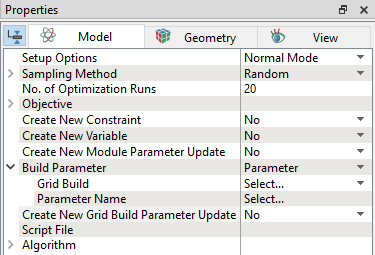
Figure 9.8 - Build Parameter
|
|
Script File: This file links Simerics software with external ones, i.e. CAD software. The commands in the files are executed at the beginning of each iteration. On linking with a script file, the following parameters are available.
- External Parameter: Allows to link the optimization variable with external parameter by selecting Add a Parameter Update from the Create New External Parameter Update drop down. On creating new External Parameter, few more parameters are available.
- Geometry Update: Allows to link the CAD Surfaces in Simerics with external geometry by selecting Add a Geometry Update from Create New Geometry Update drop down. On creating new Geometry Update, few more parameters are available.
|
|
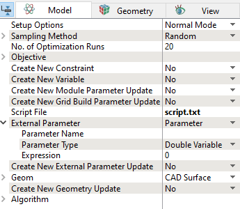
Figure 9.9 - External Parameter
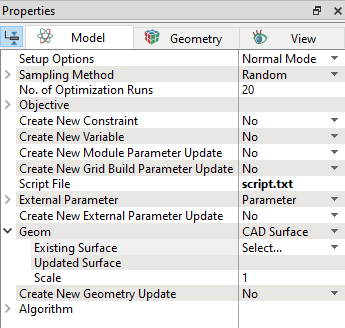
Figure 9.10 - Geometry Update
|
Algorithm
|
The list of options available under Algorithm are:
- Kernel: The Gaussian Process Regression is used to create the surrogate model. The lists of GPR kernel options available under Kernel are shown in Figure 9.11.
- Radial Basis Function (RBF):
A Radial Basis Function kernel describes any real valued function whose output depends exclusively on the distance of its input from some origin usually on a Euclidean space. - Rational Quadratic:
The Rational Quadratic kernel can be seen as a scale mixture (an infinite sum) of RBF kernels with different characteristic length scales. - Matern 3/2:
Matern kernel has an additional parameter, which controls the smoothness of the approximated function. It is less smooth compared to Matern 5/2. - Matern 5/2:
Matern 5/2 is smoother of the approximated function, when compared with Matern 3/2 and able to capture the jump in the function better. The Kernel option contains additional parameters as shown in Figure 9.11. Isotropic: If selected Yes, then it depends only on the distance of kernel arguments. Direction of deviation is of no importance. GP Noise Coefficient: The deviation from the target often experienced and intuitively it appears like a gaussian like distribution.
|
|
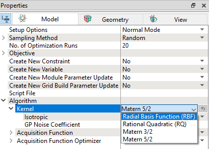
Figure 9.11 - Kernel
|
- Acquisition Function:
Acquisition Functions are techniques that guide how the parameter space must be explored during Bayesian optimization. This allows the user to choose two methods as shown in the Figure 9.12. Expected Improvement: This can be computed based on the current estimate of the Optimization performance. It considers magnitude of improvement. Probability of Improvement: It consider probability of improving current best estimate.
|
|
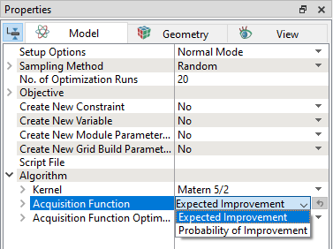
Figure 9.12 - Acquisition Function
|
- Acquisition Function Optimizer:
The optimizer finds the minimum value of the acquisition function. This allows to choose processing two options as shown in the Figure 9.13, such as
The Acquisition Function Optimizer option contains additional parameters as shown in Figure 9.13.
|
|
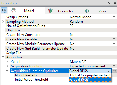
Figure 9.13 - Acquisition Function Optimizer
|


