10.2 PID Controller Template and Tutorial
Controller module in Simerics-MP+ works as a PID controller. PID controller is used in industrial control applications to regulate flow, pressure, temperature, speed, power and other process variables. This works as feedback-based control mechanism to require modulated control of a component or system. It applies a responsive correction to a control function to achieve the desired output. For example, PID controller is used to maintain the desired speed by increasing or decreasing the power output of the engine, when a car is on cruise control mode.
In this section, the parameters and settings of controller module in Simerics-MP+ are discussed in detail.
|
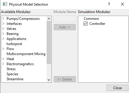
To activate the Controller module:
|
The module is explained as follows:
- Physics: Equations and constants used in the Controller module.
- Controller Parameters: Parameters used in Controller module.
- Output Variables: Outputs from the Controller module.
Physics
PID controller applies correction to a control variable  by evaluating the difference
  between the measured process variable (PV) and desired setpoint (SP). A combination of terms proportional (P), integral (I) and derivative (D) together is called as PID controller. These three control terms are varied together or in combination of two based on the application to get an accurate and optimal response. The typical workflow of PID controller is shown in the Figure 10.49.
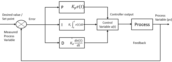
The function that governs the control variable exists in Parallel (Ideal) and Standard forms. The Parallel (Ideal) form of the control function is

|
where,
 = Control variable
 = Error between the process variable (PV) and setpoint (SP)
 = Coefficient for the proportional term (Proportional Gain)
 = Coefficient for the integral term (Integral Gain)
 = Coefficient for the derivative term (Derivative Gain)
The standard form of control function is

|
where,
 = Coefficient for the proportional term (Proportional Gain)
 = Integral time, the time sample in which the I-controller tries to eliminate the error completely
 = Derivative time, the time at which the derivative term tries to predict the future error
The behaviour of three control terms of PID are:
Proportional Term (P - Controller)
P-controller provides an output that is proportional to current value of error (SP - PV). The resulting error between the Setpoint (SP) and Process Variable (PV) is multiplied with a proportional constant ( ) to get the output. The speed of the output response depends on the proportional gain (
 ). Higher value of (
 ) results in large change in output for a given value of error and can make the system unstable. On contrast, smaller value of (
 ) makes the system less responsive for a given change in the error and for any fluctuations in the system. The P-controller always operates with a steady state error, as it is completely driven by non-zero value of error. The setpoint cannot be achieved with P-controller as the applied correction approaches zero with the error approaching to zero. In general, industrial practices suggest that the proportional term must contribute the bulk of the output response.
The response of a system to proportional gain ( ) is shown in the Figure 10.50. It can be seen with increase in (
 ), the Process Variable overshoots the Setpoint and starts oscillating.
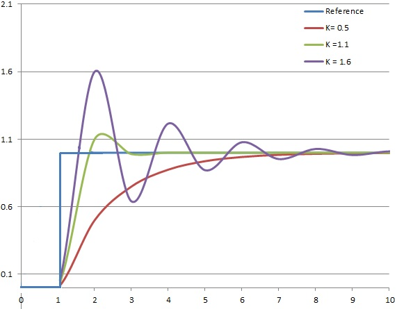
Figure 10.50 - Response of PV to step change of SP with time. ( ) and (
 ) are held constant (Source: Wikipedia)
Integral Term (I - Controller)
Integral term accounts for past values of error and integrates them over a period of time, until the error reaches zero. I-controller considers how long and how far process variable is away from setpoint, unlike the P-controller that only considers how far it is away from the setpoint. I-controller seeks to eliminate the residual error after the application of P-controller by adding a gain ( ) to the cumulative value of error. I-Controller is primarily used to reduce steady state error in the system. For many applications, P-I controllers are combined and sufficient to get a good response, accelerating to the set point with P-controller and eliminating the steady state error with I- controller. However, in the process of bringing the cumulative error to zero, I-controller can sometimes overshoot the output response as shown in the Figure 10.51.
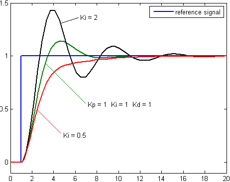
Figure 10.51 - Response of PV to step change of SP with time. ( ) and (
 ) are held constant (Source: Wikipedia)
Derivative Term (D - Controller)
Derivative term determines the slope of the error over time and multiplies it with a derivative gain  ). D-controller anticipates the future behaviour of the error based on the current rate of change and fastens the system output response. If the change is high or slope is varying continuously, high dampening effect is required to control the change. D-controller moves the control device in a direction to counteract the sudden change of the process variable. A pure D-controller cannot bring the error to zero, as it considers only the rate of change of error. It only tries to bring the rate of change to zero by damping and thereby reducing the overshoot of the output response, as shown in the Figure 10.52
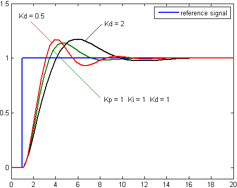
Figure 10.52 - Response of PV to step change of SP with time. ( ) and (
 ) are held constant (Source: Wikipedia)
Controller Parameters
The settings for the Controller module are as follows:
- Click Controller in the Model Panel.
- The following conditions and parameters are available in the Properties Panel.
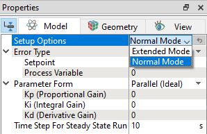
Setup OptionsThe two options available under Setup Options, as shown in Figure 10.53 are:
|
Error Type
This allows to choose the type of method to define the error.
|
|
Parameter Form
This allows to choose the form of the control function.
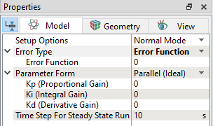
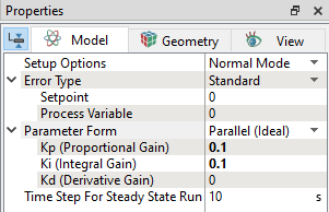
Parallel (Ideal)The ideal form of control function equation (equation 10.1) is used. The parameters required are shown in Figure 10.56
|


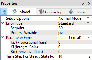
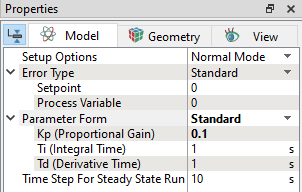
StandardThe standard form of control function equation (equation 10.2) is used. The parameters required are shown in Figure 10.57
|


| ´ | Note:  , ,  must be positive and non-zero. must be positive and non-zero. |
Initial Value
Allows to specify the initial value of the control variable.
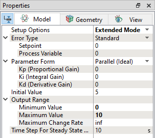
Output RangeThis is available in Advanced Mode under Setup Options. This allows to specify bounds of the control variable, as shown in Figure 10.58.
|
Time Step for Steady State Run
The time step that is used to solve the control function.
Define Control Variables
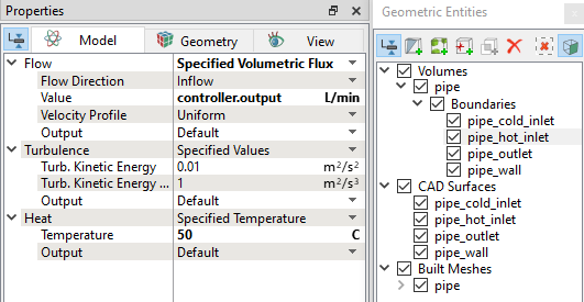
The control variable must be modified in a system to meet the desired value/set point that can be defined through expression. The syntax to define a control variable is controller.(subname).output or controller.(subname).CV. For example, flow rate at a boundary can be defined as a control variable, as shown in Figure 10.59.
Output Variables
The outputs available from the Controller module are:
-
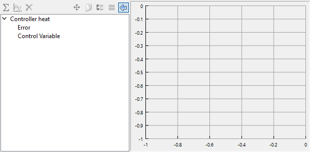
Error: This shows the difference between the measured process variable and set point over time.
- Control Variable: This shows the controller output or control variable input variation over time.
To access the list of outputs from the Controller module:
- Click Add XY-Plot
 icon in the Toolbar.
 - Click Click for Variable List
 icon to select the output, as shown in Figure 10.60.