You are here: Optimization Module and Tutorial > Optimization of 2D Shape Tutorial > Problem Overview

9.1.1 Problem Overview

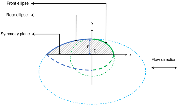
The objective of this study is to minimize the drag for a 2-D symmetric shape with a fixed height using geometry optimization. External flow simulation around the 2-D shape is performed to predict the drag. Figure 9.14 shows the geometry and the conditions for the external flow simulation. Due to the symmetric shape, only half of the model is simulated with symmetric boundary condition at the symmetry plane.

 

 

Optimization Problem Overview

The objective of this study is to minimize the drag of a 2-D structure by optimizing its geometric shape. As a basis for comparison, a circular shape is selected as the initial geometry. The first task in geometry optimization is to define the structure's geometry using a set of parameters. The geometry representation, geometric variables and constraints for optimization are described in this section.

 

Geometry Overview

The 2-D geometry is split into two parts and is represented by two elliptical curves connected at the middle point as illustrated in Figure 9.15. The upstream ellipse (represented by green color solid line) is called “Front ellipse” and downstream one (represented by blue color solid line) is called “Rear ellipse”. Each ellipse is described by a unique equation. Their centers are restricted to the y-axis but can move up and down along the y-axis. The half-height of the shape, r is fixed for both ellipses. The upper portion of the shape, depicted by the solid green and blue curves, is mirrored along the x-axis to form the complete 2-D shape as shown in Figure 9.15. This shape exhibits symmetry about the x-axis.

 

Each ellipse curve is defined by two parameters:

• The length at symmetry plane l, and
• The tip angle intercepting the symmetry plane θ (See, Figure 9.16).

 

 

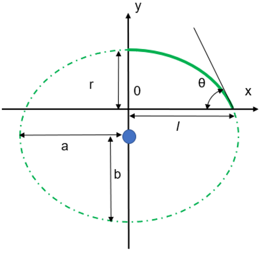
The following section derives mathematical formulations to define the geometric parameters used in the optimization. An ellipse with its center on y-axis, and a top height r can be described by:

9.5

 

where all the length scales are normalized by the height r. And a and b are minor/major axes of the ellipse.

9.6

 

9.7

 

At , where the ellipse intercepts the symmetry plane,

9.8

 

9.9

 

where, is the slope. Cotangent is used, as the range of tip angle can go up to 90 degrees. Plug into equation 9.5 and equation 9.7, we get:

 

9.10

 

9.11

 

where,

9.12

respectively.

 

Solving quadratic equation 9.11 for , we get two solutions. Notice that for angle . We pick the one with , so the center of ellipse is below the symmetry plane.

9.13

 

With the constraint as:

9.14

 

and the corresponding limit for the angle is:

9.15

 

Geometric variables

As shown in Figure 9.16, each ellipse is defined by a length l and a tip angle θ. Hence there are four geometric parameters that can be modified to attain an optimized shape. The four parameters are front length fl, front angle fa corresponding to front ellipse and rear length rl, rear angle ra corresponding to rear ellipse. These variables are varied in a range as defined below.

 

1. The range for front and rear length is 0.5 - 8, normalized by the half-height r.

2. The range for front and rear tip angle is 10-90 deg.

 

Constraints

Constraints for the geometrical parameters are specified to avoid invalid or undesired geometries during the optimization process. In this case, the same constraints are specified for both of the tip angles, as described in equation 9.15.