Discrete Particle Model
Within the discrete particle model, the flow of the dispersed phase is modelled by tracking a specified number of particles through the continuous fluid phase. In Simerics-MP, the model has the following assumptions/restrictions:
-
The discrete phase is composed of definite number of spherical particles through the continuous fluid flow phase. The particles are defined to be either having a mass, Has Mass or Massless.
-
The size of a particle is determined by a specified radius at the release position and time and remains unchanged. The particle-particle interaction is assumed to be negligible.
-
The particles interact with both the fluid flow and wall boundaries, but the volume of a particle neither displaces any fluid (low volume fractions in the particle phase) nor interferes with the geometry (i.e. an oversize particle could fit through a smaller gap).
-
Between the continuous fluid phase and the particles there are no heat and mass transfer. The particle temperature is assumed to be the same as the local temperature of the fluid flow.
Under these assumptions, the motion of each individual particle is tracked using a Lagrangian approach. The tracking is carried out by forming a set of ordinary differential equations in time for each particle, consisting of equations for position and velocity. These equations are then integrated over time to calculate the behavior of the particles as they traverse the flow domain. The particle modelling approach in Simerics-MP has the following salient characteristics:
-
The discrete particle model follows the Euler-Lagrange approach. The fluid phase is treated as a continuum by solving the continuity and Navier-Stokes equations, while the dispersed phase is solved by tracking the motion of each individual particle using a Lagrangian approach. The fraction of volume taken by the particles is not included in the continuous phase calculation.
-
For the option of Massless, the particles are moving along with the fluid flow, or following the streamlines of the flow field. In this case, the size (radius) of the particles does not have any influence on both the flow and particles and is used for the purpose of display only.
-
For the particles with mass (Has Mass), the mass of a particle is dictated by the specified particle radius/ diameter and particle density. The forces acting on a particle, which determine the motion of particles, include particle-fluid drag (inertial force) and gravity. The turbulence dispersion forces on particles are not considered. In this option, the size of the particles influences both the particle-fluid drag forces as well as post processing.
-
The momentum exchange between the fluid phase and the discrete particle phases are modelled by one-way coupling in which only the fluid phase affects the motions of particles or two-way coupling where the particles also affect the fluid flow through particle-fluid drag forces.
-
The wall-particle interactions are modelled using a variety of particle wall models including stick, perfect bounce and partial bounce.
-
While the fluid phase can be both steady and unsteady, the particle tracking is a transient process that involves the integration of particle paths through the discretized domain. In this approach, individual particles are released/injected from the specified locations at different times. Each particle is then tracked from its release position to final destination (either escapes the domain or meet certain integration limits). Finally, an average of all particle tracks can be obtained, and the particle-fluid interactions are calculated as source terms to the fluid phase momentum equations.
-
The path travelled by particles can be displayed using the related Streakline Tracking Method available in the Particle module.
Particle Motion Theory
In the Lagrange approach, the particle motion is determined by the force balance on the particle and the conditions under which the particle is released (initial conditions). To model the discrete particle phase, therefore, the equations of motion for particles are first formed based on force balance. Then the boundary and initial conditions for particles are specified. Finally, the integration of particle equation of motion is carried out for particle tracking.
Equations of Motion for Particles
Particle Force Balance
For a discrete particle traveling in a continuous fluid medium, the motion of the particle is determined by the net force acting on it. According to Newton’s second law, the force balance on the particle can be written in the following Lagrange form:

|
where

|
Particle mass (kg) |

|
Particle velocity (m/s) |

|
Net force exerted on the particle (N), which affects the particle acceleration. |
In a Cartesian coordinate system, let point  represent the location of the particle, and
  be the particle velocity components. With the Lagrangian approach, the particle velocity
  is defined as:

|
For a spherical particle occupying a volume  with density
  and diameter
  (Simerics-MP accepts radius as input), the particle mass
  is computed as:

|
As for the net force  there are a number of contributing factors such as, the fluid-to-particle drag force, the gravity effect, the forces due to domain rotation (centripetal and Coriolis forces), and other forces due to the difference in velocity between the particle and fluid as well as to the displacement of the fluid by the particle. In Simerics-MP
 may be expressed as follows:

|
where

|
Drag force (N) |

|
Gravity force (N) |

|
Centripetal and Coriolis forces (N) |

|
Other forces such as virtual mass force, pressure gradient force, lift force, etc. specified by the user (N) |
By default, only the drag force on the particle is considered.
Substituting equation 5.516 into equation 5.513 and dividing it by  , the solved force balance equation for a particle has the following form:

|
To close equation 5.517, the contribution of each individual force needs to be calculated. The sub-models or formulations adopted in Simerics-MP are described in the following subsections.
Drag Force on Particles
The aerodynamic drag force on a particle is proportional to the phase slip velocity, the difference between the fluid and particle velocities. Assuming that at the same space where the particle is located at a given time, the fluid flow velocity equals  , then we have the drag force in the form:

|
where  is the fluid phase density; and
  is the area of the particle projected in the flow direction. For a spherical particle with diameter
  ,
,  is the maximum area of cross section:

|
The term  is the drag coefficient, which depends on the relative Reynolds number,
  :
:

|
where  is the fluid dynamic viscosity (Pa-s).
The drag coefficient  is introduced to account for experimental results on the viscous drag of a solid sphere. Various models or empirical correlations have been developed to determine the drag function
  (
( ) to estimate the fluid-particle exchange. For smooth spherical particles, among many models, the most complete
  function is the corrections by Morsi and Alexander1S. A. Morsi and A. J. Alexander, "An Investigation of Particle Trajectories in Two-Phase Flow
Systems", J. Fluid Mech., 55(2) 193–208, September 26 1972., which has the general expression:
function is the corrections by Morsi and Alexander1S. A. Morsi and A. J. Alexander, "An Investigation of Particle Trajectories in Two-Phase Flow
Systems", J. Fluid Mech., 55(2) 193–208, September 26 1972., which has the general expression:

|
where  ,
,  and
and  are model constants, whose values depend on the relative Reynolds number, as shown in Table 5.42.

|

|

|

|
|---|---|---|---|
0 <  <=0.1 <=0.1 |
0 | 24 | 0 |
0.1 <  <=1 <=1 |
3.690 | 22.73 | 0.0903 |
1<  <=10 <=10 |
1.222 | 29.1667 | -3.8889 |
10 <  <=100 <=100 |
0.6167 | 46.50 | -116.67 |
100 <  <=1000 <=1000 |
0.3644 | 98.33 | -2778 |
1000 <  <=5000 <=5000 |
0.357 | 148.62 | -47500 |
5000 <  <=10000 <=10000 |
0.46 | -490.546 | 578700 |
 >10000 >10000 |
0.5191 | -1662.5 | 5416700 |
From Table 5.42, one can see that at very low particle Reynolds numbers (the viscous regime),  , the drag coefficient for flow past spherical particles returns to the Stokes’ law:

|
On the other hand, when  is sufficiently large so that the inertial effects dominate the viscous effects, the fluid-particle flow is in the inertial or Newton regime. From Table 5.42, it is clear that the drag coefficient becomes less and less dependent on the relative Reynolds number. In fact, a constant of
  value is often used instead of the full Morsi and Alexander model:

|
In the transitional region between the viscous and inertial regimes,  , for spherical particles, both viscous and inertial effects are important. Therefore, the drag coefficient is a complex function of the relative Reynolds number, which can be estimated by Morsi and Alexander model or other correlations. For example, according to the Schiller and Naumann model2L. Schiller and Z. Naumann, "Z. Ver. Deutsch. Ing. 77. 318. 1935.:

|
Finally, to simplify the expression of the drag force term in equation 5.517, the “particulate relaxation time”,  , is introduced:

|
By combing equations equation 5.515, equation 5.518 - equation 5.520 and equation 5.525, the drag force per unit particle mass has the formulation:

|
|

|
|

|
Therefore, the default (only the drag force is considered) particle force balance equation has the form:

|
Inclusion of the Gravity Term
The gravity term is by default not included in the particle force balance equation. However, it can be turned on as an option in Simerics-MP. For a particle immersed in fluid flow, the effect of gravity results in a buoyancy force, which is equal to the weight of the displaced fluid by the particle. Assuming  is the fluid mass displaced by the particle and
  is the gravity vector, the resulting force is given as:

|
Or the force per unit particle mass is given as:

|
And the force balance equation has the form:

|
Rotation Force on Particles
When modelling fluid flows in a rotating reference frame, the rotation-induced additional force term,  , is an intrinsic part of the particle acceleration and consists of the effect of Coriolis and centripetal forces:

|
|

|
Or the rotation force per unit particle mass is given as:

|
where  is the angular velocity of the rotating reference frame and
  is the vector connecting the axis center and particle location. With the addition of this force term, the particle balance equation is:

|
equation 5.533 governs the motion of a particle in a Lagrange system when the flow is solved in a rotating reference frame.
Boundary and Initial Conditions for Particles
In the Lagrange approach, particle tracking is a transient procedure. Therefore, both boundary and initial conditions are required to calculate the trajectories of the particles. The boundary conditions define the particle behavior at the boundaries of the computational domain, in particular, the particle-wall interactions. The initial conditions concern the particle release from boundaries including the release position, frequency, velocity, particle type and size (radius), and the number of particles. In this section, both the initial and boundary conditions are described.
Boundary Conditions
Simerics-MP applies a discrete phase boundary condition to determine the behavior of particles at a boundary. When a particle reaches a boundary of the flow domain (including physical boundary and solid-fluid interface), for example a wall or an inlet boundary, one of several scenarios may occur at the boundary:
- The particle may be reflected via an elastic or inelastic collision.
- The particle may escape through the boundary. In such a case, the particle is lost from the calculation at the point of impact with the boundary.
- The particle may be trapped at the wall and is lost from the calculation at the point of impact with the boundary.
- The particle may pass through an internal boundary zone, such as fan or porous jump.
- The particle-boundary interaction may also be determined by user-defined methods to model the particle behavior when hitting the boundary.
Based on the particle behavior at boundaries, the flow boundary conditions and interfaces are regrouped into three types of discrete particle boundary conditions: Open, Symmetry and Wall.
Open Particle Boundary
Open discrete boundary condition allows particles or streamlines to exit the computational domain. For the discrete particle phase, an open boundary is usually an inlet or outlet boundary of the fluid flow phase in the Euler system, but it can also apply to the other types of flow boundaries such as wall and symmetry. At an open particle boundary, the particle can either leave from or enter into the domain depending on the particle velocity direction.
Let  be the unit normal vector to the open boundary which points in the direction away from the computational domain, with the particle boundary velocity
  . If
. If  , the velocity vector
  points away from the computational domain, indicating that the particle escapes through the boundary. The particle is then lost from the calculation at the point of impact with the boundary.
Symmetry Particle Boundary
When a particle or streakline in the computational domain hits a discrete symmetry boundary, the boundary condition only allows it to reflect back into the domain. For the discrete particle phase, a symmetry particle boundary typically corresponds to a flow symmetry in the Euler system. It can also be served as a location for particle release.
Let  be the normal-to-symmetry unit vector at point “
 ” of the symmetry, with its direction pointing away from the symmetry to the computational domain. Further,
  and
and  are introduced to indicate the particle impact velocity angle at the particle symmetry boundary, as shown in Figure 5.215. With the particle reflecting from the symmetry, its total kinetic energy is conserved: the tangential velocity remains the same while the normal velocity component only changes the sign. Mathematically, the particle symmetry boundary condition can be expressed as:

|
where

|
Angle at the point “ |

|
Magnitude of particle incident velocity (m/s) |

|
Magnitude of particle reflected velocity (m/s) |
 ": of the symmetry (
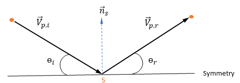
Wall Particle Boundary
Particle-wall interaction involves very complex physical phenomena and not all aspects are well understood. For example, for liquid droplets, dimensional analysis shows that the droplet-wall interaction depends on the wall temperature, wall material and roughness, impact angle and impact velocity, the existence of a wall film, and various other parameters. As a result, there are a range of sub-models developed to reproduce the different regimes of wall-particle interactions as well as to account for the impacts of flow parameters and wall boundary conditions.
In the present discrete particle model, the shape, size and mass of the particles are assumed to remain unchanged. Also, the fluid and particles are considered to be in thermal equilibrium. Therefore, a very simplistic approach is used to describe the process of particles (has mass) colliding with walls: During the collision process, particles exchange momentum only with the wall, and the particles can only have one of three ways to interact with the wall: perfect bounce, stick and partial bounce, as shown in Figure 5.216.
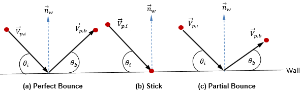
Figure 5.216 - Particle - wall interactions
Perfect Bounce: As shown in Figure 5.216 (a), the perfect bounce wall boundary condition acts in the same way as the symmetry boundary: a particle or streakline reflects when it hits a wall. The momentum and kinetic energy of the particle is perfectly conserved, and the angle of incidence is equal to the angle of reflection, but the wall normal velocity component changes sign:

|
where

|
Wall normal unit vector |

|
Angle at the wall boundary (deg) |

|
Magnitude of the particle incident velocity (m/s) |

|
Magnitude of the particle bounce velocity (m/s) |
Stick: As shown in Figure 5.216 (b), when a particle collides with the wall, it loses all its momentum and energy and sticks to the wall:

|
Without the consideration of the particle accumulation along the wall, the particle is then completely lost from the calculation at the point of impact with the boundary.
Partial Bounce: As shown in Figure 5.216 (c), the partial bounce is a wall particle condition between the perfect bounce and stick: A particle or streakline bounces from a wall but with the loss of part of the energy in normal and/or tangential direction. In this condition, the momentum and kinetic energy of the particle is not conserved, and the angle of incidence is usually larger than the angle of reflection:

|
The loss of energy through particle-wall interaction is specified by user-inputs:
- Normal Energy Loss: It specifies the loss of the normal component of kinetic energy of a particle on the wall.
- Tangential Energy Loss: It specifies the loss of the tangential component of kinetic energy of a particle on the wall.
In Simerics-MP, whether a particle will bounce, or stick is decided by the specified values of the maximum and minimum normal velocities. Assuming that  and
and  are the specified particle maximum and minimum normal velocities respectively, we have the following conditions:
- If
 or
or  , the particle will bounce from the wall.
 - If
 , the particle will stick to the wall.
Finally, it may be stressed that the particle-wall interaction models only apply for the particles Has mass. For a massless particle, it follows the flow streamline along the walls.
It may also be noted that the particle wall boundaries can be the external walls and fluid-solid interfaces. As in the open and symmetry particle boundaries, particles can be released from a wall boundary.
Initial Conditions (Release Particles)
The initial conditions provide the starting values for all of the dependent discrete phase variables that describe the instantaneous conditions of an individual particle. For the Lagrange particle tracking, the procedure to determine initial conditions involves particle releases (frequency and distributions) from boundaries (open, symmetry, wall and interface), and assigning properties for each particle.
With the activation of Release Particle, the following parameters/variables are described to serve as the initial conditions for the particle motions:
Integration of Particle Equation of Motion
To track the particle motion, the trajectory equations of each particle are solved (integrated) either analytically or numerically in a Lagrange system. From equation 5.514 and equation 5.533, the motion equations may be rewritten as:

|
|

|
where  is the position vector of the particle; and
  includes accelerations due to all other forces except drag force (e.g., gravity, rotation effects).
equation 5.538 and equation 5.539 are set of coupled ordinary differential equations. With given initial and boundary conditions, the particle displacement, equation 5.538, is calculated using the forward Euler integration of the particle velocity over time-step,  :
:

|
where the superscripts  and
and  refer to the new and current values respectively, and
  is the particle velocity at the current time-step. At the first time-step,
  and are the release position and initial velocity, respectively:

|
In this forward integration method, the particle velocity calculated at the start of the time-step is assumed to prevail over the entire step. At the end of the time-step, the new particle velocity is calculated by solving the particle momentum equation 5.539. Assuming that  ,
,  and
and  are constant over the time period
  , and the fluid properties are taken from the start of the time-step (at the time
  ), we have the analytical solution of equation 5.539:

|
It may be noted that to evaluate  and
and  , fluid variables such as density, viscosity and velocity are needed at the position of the particle. They are taken as the cell values of the fluid flow phase in which the particle is currently located. It may also be pointed out that this analytic scheme is very efficient. However, it can become inaccurate for large time steps and in situations where the particles are not in hydrodynamic equilibrium with the continuous fluid flow. In such a case, the numerical schemes can be used to integrate the equation 5.539.
Particle-Fluid Coupling
In the Euler-Lagrange approach, the continuous fluid flow is assumed to always affect the particle behavior through forces, heat and mass transfer. For example, the force term  in the particle force balance equation 5.517 concerns the aerodynamic drag force of flow on the particle. Though the particle phase is considered to be discrete and does not displace the fluid in volume, the particles can exert a counteracting influence on the fluid flow through the exchanges of momentum, and possibly mass and heat. The effect of the particles on the flow is commonly referred to as particle-fluid coupling. In numerical simulations, the particle-fluid coupling is further classified into two categories: one-way coupling and two-way coupling.
One-Way Coupling
One-way coupling only allows the fluid to influence trajectories of particles, but particles do not have any effect on the fluid. For massless particles, the particle-fluid interaction is always one-way coupling: the particles move along with the fluid flow. For particles has mass, one-way coupling may be an acceptable approximation in flows with low dispersed phase loadings where particles have a negligible influence on the fluid flow.
With one-way coupling, the numerical prediction of fluid-particle two-phase flows is pretty straightforward. For the continuous fluid phase, the flow field is calculated as a single-phase fluid flow without the existence of dispersed particle phase. The particle motion is then tracked based on the computed flow filed and the initial conditions. For a steady-state flow, the particle-tracking occurs only once after the converged flow solution of the continuous phase is obtained by solving the continuity and Navier-Stokes equations. For a transient flow simulation, the particle motions are tracked only at the end of each time-step of the flow simulation.
Two-Way Coupling
For particles with mass (Has Mass), the two-way coupling not only allows the fluid to influence trajectories of particles, but also accounts for the effect of particles on the continuous fluid phase. Without the inclusion of the mass and heat transfer, the two-way interaction between the fluid and particles only concerns the momentum exchange. For the momentum transferred from the continuous phase to the discrete phase, it is computed by tracking the momentum gained or lost by each individual particle as they pass through a control volume. In two-way coupling, the particle-fluid momentum exchanges are required to be included in the fluid momentum equations to account for the effect of the discrete phase trajectories on the continuum. From equation 5.533, among the three particle forces considered (drag, gravity and rotation), only the drag force accounts for the particle-fluid momentum exchange and is thus added in the momentum equations. Note that for Massless particles, no interchange terms are computed between the fluid flow and the massless particles, so that the discrete phase trajectories have no impact on the continuum.
To include the particle-fluid drag effects in the continuous phase momentum equations, the drag force for each particle moving through the flow is applied in the control volume where the particle is located during the time-step. Specifically, for the particle, “ ”, its momentum source due to drag,
  , is calculated from the following ordinary differential equation:

|
And the particle source to the continuous phase is the source term  multiplied by the number flow rate for that particle (the mass flow rate divided by the mass of the particle):

|
where  is the time-step; and
  is particle mass flow rate.
Assuming that  is the number of particles passing through a control volume at the time-step
  , we have the total particle-to-fluid source term:

|
With the addition of the fluid-particle drag force, the governing equations solved for the continuous phase have then following form:

|
|

|
Clearly, with one-way coupling,  , the continuous fluid phase is governed by the exact single-phase continuity and momentum equations. For two-way coupling, the only difference is the additional particle-to-fluid drag force source term. equation 5.546 and equation 5.547 are solved in the same way as the single-phase flow.