Simerics-MP applies a streamline boundary condition to determine the behavior of flow streamlines at a boundary. When streamlines are at a boundary of the flow domain (including external boundaries and solid-fluid interfaces), for example a wall or an inlet boundary, one of several scenarios may occur at the boundary:

• The streamlines may be reflected.
• The streamlines may enter, leave or both enter and leave through the boundary.
• The streamlines may pass through an internal boundary zone, such as fan or porous jump.

Based on the streamline behavior at the boundaries, the flow boundary conditions and flow-solid interfaces are regrouped into three types of streamline boundary conditions: Open, Symmetry and Wall.

Open Streamline Boundary

Open streamline boundary condition allows streamlines to exit, enter, or both exit and enter the computational domain. An open boundary is usually an inlet or outlet boundary of the fluid flow, but it can also apply to the other types of flow boundaries such as wall and symmetry. At an open boundary, the streamline can either leave from or enter into the domain depending on the particle (flow) velocity direction.

Let be the unit normal vector to the open boundary which points in the direction away from the computational domain, with the particle boundary velocity (the same as the flow velocity at the point) we have the following streamline conditions at the open boundary:

• If , the velocity vector points away from the computational domain, indicating that the particle/flow escapes through the boundary. The particle is then lost from the flow domain at the point of impact with the boundary.
• If , the velocity vector points to the computational domain, indicating that the particle/flow enters into the domain from the boundary. This particle is released/injected into the fluid flow from the open boundary along with the inflow. The particle is a part of the streamline calculation at the point of impact with the boundary.

Symmetry Streamline Boundary

At a streamline symmetry boundary, the streamlines are reflected at the boundary. For streamlines, a symmetry boundary typically corresponds to the flow symmetry. It can also be a location for particle release/escape in the same way as in the open streamline boundary.

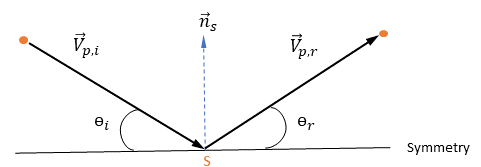
Let be the normal-to-symmetry unit vector at point “” of the symmetry boundary, with its direction pointing away from the symmetry towards the computational domain. Further, and are introduced to indicate the angle of the particle impact velocity (local flow velocity) at the symmetry streamline boundary, as shown in Figure 5.247. With the particle reflecting from the symmetry boundary, the tangential velocity remains the same while the normal velocity component only changes the sign. Mathematically, the particle/streamline symmetry boundary condition can be expressed as:

5.567

where and are the particle reflecting velocity and angle at the point “" of the symmetry boundary respectively; and and represent the velocity magnitudes.

Note that since the massless particles travel at the local flow velocity, which is obtained by flow simulations, no boundary condition is required when equation 5.566 is integrated at a streamline symmetry boundary.

Wall Streamline Boundary

For streamlines, a wall streamline boundary typically corresponds to the wall flow boundary. At a streamline wall boundary, the massless particles move with the fluid flow. Since the local flow velocity, thus the particle velocity, is obtained using the appropriate near-wall models, no explicit wall boundary condition is required to solve equation 5.566.

It may also be noted that the streamline wall boundaries can be the external walls and fluid-solid interfaces. As in the open and symmetry streamline boundaries, a wall streamline boundary can also be served as a location for particle releases.