This tutorial includes:
This tutorial teaches you how to:
Set machine data and load curve files independently.
Specify a “cut-off or square” edge on a blade.
Choose an appropriate topology family under ATM Topology.
Change the distribution of mesh elements along a cut-off edge.
As you work through this tutorial, you will create a mesh for a blade passage of a radial compressor blade row. A typical blade passage is shown by the black outline in the figure below.
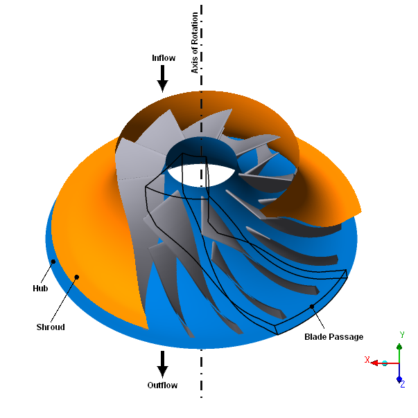
The blade row contains 9 main blades and 9 splitter blades that revolve about the negative Z axis. The blades have cut-off trailing edges. A clearance gap exists between the blades and the shroud, with a width of 5% of the total span. Within the blade passage, the maximum diameter of the shroud is approximately 125 mm.
If this is the first tutorial you are working with, it is important to review Introduction to the Ansys TurboGrid Tutorials before beginning.
Create a working directory.
Ansys TurboGrid uses a working directory as the default location for loading and saving files for a particular session or project.
Download the
radcomp.zipfile here .Unzip
radcomp.zipto your working directory.Ensure that the following tutorial input files are in your working directory:
BladeGen.inf
profile.crv
hub.crv
shroud.crv
Set the working directory and start Ansys TurboGrid.
For details, see Setting the Working Directory and Starting Ansys TurboGrid.
In the Rotor 37 tutorial, you loaded a BladeGen.inf file in order to specify the machine data (# of blade sets,
rotation axis, and units) and the hub, shroud, and blade curve files.
In the Steam Stator tutorial, you entered the same data using the Load Profile Points Or CAD command. In this tutorial, you will define
the machine data and curve files individually, by editing the corresponding
geometry objects.
Set up the Machine Data object, which contains
basic information about the geometry:
In the Mesh workspace, open
Geometry>Machine Data.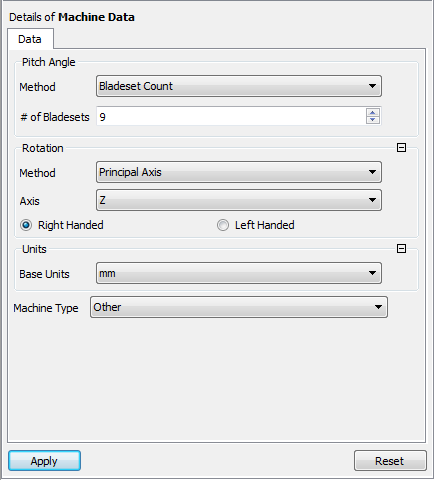
Set # of Bladesets to
9.Set Base Units to
mm.Click Apply to save the settings.
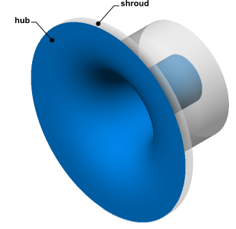
Open
Geometry>Hub.Set Length Units to
mm.Ensure that File Name is set to
./hub.crvfrom your working directory.Click Apply.
Open
Geometry>Shroud.Set Length Units to
mm.Ensure that File Name is set to
./shroud.crvfrom your working directory.Click Apply.
Note: If you had loaded the
BladeGen.inffile, the Curve Type settings for theHubandShroudobjects would have been set toPiece-wise linearinstead of the default:Bspline. Either setting will work for this geometry.
At this point, the entire hub and shroud surfaces are shown. After a blade is defined (in the next step), the hub and shroud will be trimmed to show only one passage.
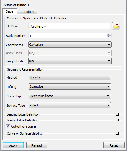
In the Mesh workspace, open
Geometry>Blade Set>Blade 1.Ensure that File Name is set to
./profile.crv.Set Length Units to
mm.Set Geometric Representation > Method to
Specify.Set Geometric Representation > Lofting to
Spanwise.Set Geometric Representation > Curve Type to
Piece-wise linear.Set Geometric Representation > Surface Type to
Ruled.Under Trailing Edge Definition, select Cut-off or square.
Click Apply.
The progress bar at the bottom right of the screen shows the geometry generation progress. After the geometry has been generated, you can see the hub, shroud, and blade for one passage. Along the blade, you can see the leading and trailing edge curves (green and red lines, respectively).
Right-click
Geometry>Blade Setand select Insert > Blade.Click to accept the default name.
Set Blade Number to
2.Click Apply.
To complete the geometry, create a small gap between the blade and the shroud. The blade should be shortened to 95% of its original span because the gap width is 5% of the total span, as specified in the problem description.
Open
Geometry>Blade Set>Shroud Tip.Set Tip Option to
Constant Span.Set Span to
0.95.Click Apply.
In this tutorial, you will manually choose a set of ATM topology templates, called a topology family.
Click the Topology Viewer tab.
Open
Topology Set.Browse through ATM Topology > Method.
ATM Topology > Method provides a list of topology families from which you can manually choose. When you mouse over or cursor through the list, the Topology Viewer shows a picture of the highlighted topology family and a description of the type of blade that the family best fits.
Set ATM Topology > Method to
Single Splitter.Click Apply to set the topology.
Right-click
Topology Setand turn off Suspend Object Updates.The topology and 3D mesh are generated.
The Mesh Data object indicates that there is a problem with mesh quality.
Click the 3D Viewer tab.
Expand the
Mesh Dataobject in the object selector.Open one of the
Boundary Layer Controlobjects underMesh Data.
Note that the near wall expansion rate is outside the established limit within the boundary layer region. The affected mesh regions are colored red in the viewer.
Add more elements to the boundary layer region as follows:
Open the
Mesh Dataobject.On the Mesh Size tab, ensure that Boundary Layer Refinement Control > Method is set to
Proportional to Mesh Size.Set Boundary Layer Refinement Control > Parameters > Factor Base to
4.0.Click Apply.
The Mesh Data object no longer indicates that there is a problem with
mesh quality.
As an exercise, change the distribution of elements across the cut-off edge as follows:
Set Cutoff Edge Split Factor > Trailing to
0.9.Click Apply.
Note that, for a blade that has one rounded edge and one cut-off edge, the distribution of elements across the blade tip mesh is governed by the distribution across the cut-off edge.
Check the 3D mesh statistics:
Open
Mesh Analysis.The mesh statistics are acceptable based on the current quality criteria.
Close the Mesh Statistics dialog box.
Save the mesh:
Click File > Save Mesh As.
Ensure that Files of type is set to
Ansys CFX Mesh Files.Set Export Units to
cm.Set File name to
radial_compressor.gtm.Ensure that your working directory is set correctly.
Click Save.