Motions of a Rigid Body
In CFD simulations, the surfaces of a solid object usually serve as wall boundaries in a flow domain. When a solid object or surface is subjected to dynamic and mechanical forces, and thermal effect, the imbalance of the net forces can cause the body to move and deform. Without getting into detailed analysis of the fluid-structure interactions or explicitly described motions and/or deformations, a solid object is often considered as a rigid body in flow simulations. Therefore, for a solid object subjected to force imbalances, it is assumed that it can move linearly (translation) and/or angularly (rotation) without deformation. For a CFD computational domain, however, the boundary movement can lead to the domain change and consequently, the volume mesh may deform, as described in Flow module.
For a rigid body, the equations governing its motions are derived directly from the conservation of linear and angular momentum:
Linear Momentum (Translation)

|
Angular Momentum (Rotation)

|
In equation 5.573,  is the mass of the moving object;
  ⃗ is the linear/transitional velocity; and
  ⃗ is the total/net forces exerted on the body under translation. In equation 5.574,
  is the moment of inertia;
  ⃗ is the angular velocity; and
  ⃗ is the total/net torque acted on the rotating body.
equation 5.573 and equation 5.574 govern the general motions of a solid body, which have six degrees of freedom (6-DOF) with three each for translation (3-DOF) and rotation (3-DOF), respectively. At present, only 1-DOF translation and rotation are considered In Simerics-MP, which will be presented in the following sections.
One-DOF Translation
 Description
With the assumption that a solid body moves linearly in an arbitrarily specified direction (remain unchanged), defined by a unit vector, , the translational motion of the body is reduced to be one degree of freedom (1-DOF). As a result, for the linear momentum conservation, equation 5.573 becomes a scalar equation along the moving direction since the moving velocity and force can be expressed in terms of
  :
:

|

|
|

|
where  is the magnitude of the position vector
  ⃗ at a point of interest (on the solid body) along the moving direction,
  . In a Cartesian coordinate system, we have

|
If the mass of the solid body remains a constant, and then expanding the force term to explicitly include all the forces applied on the body, we have the scalar linear momentum equation as:

|
The forces on the right-hand side indicate the following:
Hydrodynamic Force
The hydrodynamic force,  , consists of pressure and shear forces, caused by the relative motion between the fluid flow and the surfaces of the solid body which are in contact with the flow. The pressure and shear forces are obtained from the flow solutions (output quantities):

|
Damping Force
The damping force,  , is a retarding force caused by the frictional damping effect. It is decided by the motion of the solid object and the specified (user-defined) damping coefficient,
  :
:

|
Spring Force
The spring force  , depends on the displacement of the string (
 ), spring constant (
 ), and the spring preload force (
 ):
):

|
where the spring displacement  , is defined as:

|
where  is the magnitude of the position vector
  at previous location,
  .
.
Friction Force
The contact friction model is adopted to account for the effect of friction in a dynamic system. The friction force  , is modelled as:

|
where  is the normal component of the contact force exerted on the solid surface of interest. And for friction coefficient
  , the static friction coefficient
  , and the sliding friction coefficient
  , are further introduced for the stationary and moving bodies, respectively:

|
Additional Force
 is added for additional user-specified forces.
One-DOF Rotation
Description
As in the 1-DOF translation, when an arbitrary rotating axis is defined by a point (center of the axis)  , and the directional unit vector,
  , the solid body rotation around the axis
  is also reduced to 1-DOF rotation. Similarly, for the angular momentum conservation, equation 5.574 also becomes a scalar equation along the tangential direction
  , defined as:

|
where  is the vector pointing from the center of the axis
  to an arbitrary point
  on the solid body:

|
The angular velocity and torque at the point  can be rewritten as:

|
|

|
|

|
where  is the angle of rotation of the point
  relative to the starting/reference location.
If the moment of inertia remains a constant, and expanding the torque term to explicitly include all the torques applied on the rotating body, we have the scalar angular momentum equation as:

|
The torque terms on the right-hand side are defined as follows:
Hydrodynamic Torque
The hydrodynamic torque,  , is the combination of torque due to pressure and shear forces:

|
Damping Torque
The retarding torque due to damping,  , depends on the rotational speed
  and the specified (user-defined) damping coefficient,
  :
:

|
Spring Torque
The torque  , induced by torsion, depends on the displacement angle, (
 ), and the user-defined preload torque
  , and the torsion constant
  .
.

|
where  is the reference angle. It is typically the position of the boundary or volume during the model set up (or a valve’s closed position for the Valve Template in Simerics-MP+) but can correspond to a different location. For example, at zero angular displacement, the reference angle
  is not the same as the initial angular position.
Friction Torque
Friction torque is the torque caused by the frictional force that occurs when two objects in contact move. In experiments, it is determined by the difference between the applied torque and observed/net torque. It depends on the friction coefficient ( ) and the contact torque due to the normal force (
 ) applied on the contact surface:

|
where  is a user-defined parameter, which is defined as in equation 5.585.
Additional Torques
 is added for additional user-specified torques.
Bounce Model
Description
In many situations, a solid body can only translate and/or rotate in a limited space (limited distance or angle), namely, it has a maximum and/or minimum position. For example, as shown in Figure 5.268, when a simple gravity pendulum is released from the original position with the angle  , the restoring force acting on the its mass causes it to oscillate about the equilibrium position. The maximum angle on either side of the equilibrium position (
 ) depends on its releasing position,
  . If there is no friction (frictionless pivot and in vacuum), the maximum angle will remain unchanged and the pendulum would swing back and forth permanently with the same extreme positions. However, when a pendulum is in the atmosphere, for instance, the air resistance (damping) would cause the maximum swinging angle to reduce with time and eventually it will stop at the equilibrium position.
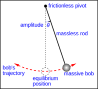
Furthermore, in a swinging cycle (period), when the pendulum reaches the highest position  , it changes direction with the total loss of its kinetic energy: in the simple gravity pendulum, the kinetic energy is completely transferred into potential energy, while when the resistance of the medium is considered, a part of the kinetic energy is lost to overcome the viscous damping. However, the net force or the potential energy drives the pendulum to start moving in the opposition direction towards the equilibrium position, where the kinetic energy (speed) is the maximum while the potential is the lowest. In this case,
  indicates a “no bounce” condition for the 1-DOF angular momentum equation 5.591.
In addition to the so-called “no-bounce” condition, a moving body at the limiting position may not lose any kinetic energy at all and bounce back (perfect bounce), or only lose a part of its kinetic energy (partial bounce). Therefore, in Simerics-MP, the follow three “bounce” conditions are applied when the 1-DOF dynamics equations of translation and rotation, equation 5.579 and equation 5.591, are solved to determine the motions of a solid body or a wall boundary for the flow domain:
No Bounce
This is the default model in Simerics-MP. This dictates that when a solid body/boundary reaches the limit of its motion, it changes direction with the total loss of its kinetic energy. With the subscripts, “ ” and “
 ” representing bounce and incidence, and
  and
and  are translational and rotating speed (magnitude only), this bounce model can be expressed as follows:
Translation

|
Rotation

|
Partial Bounce
The partial bounce model dictates that when a solid body/boundary reaches the limit of its motion, it changes direction with the partial loss of its kinetic energy, determined by a user-specified factor,  :
:
Translation

|
Rotation

|
Perfect Bounce
The perfect bounce model dictates that when a solid body/boundary reaches the limit of its motion, it changes direction with zero loss of its kinetic energy,  :
:
Translation

|
Rotation

|