Flow Models
The properties and the conditions for the flow solution are specified based on different models as explained in this section:
- Density Models
- Viscosity Models
- Deformation Model: Used to model complaint wall boundaries
- Resistor Capacitor Model: Used to model boundaries or interfaces, with existing loads on the system
- Porous Media Resistance Model: Used to model flow with obstructions (porous media)
Density Models
Density ( ) is a material property defining the state of a fluid flow as incompressible or compressible. The constitutive equation of state for density has the general form:

|
where  is the absolute pressure and
  is temperature. The unit for density is kg/m3.
In Simerics-MP, in addition to the user-defined density law using “Expression Editor”, several special constitutive equations of state are given to determine the flow density in order to close the flow governing equations.
Constant Density
In a fluid flow, the assumption of constant density simplifies the flow as incompressible. For most liquids, the density can be considered constant unless it shows significantly large variations with pressure and/or temperature.
Compressible Liquid
In many applications such as water hammers and fuel injectors, the compressibility effects of a liquid are essential to decide the flow characteristics and thus the performances of the flow components/equipment. To account for the density compressibility, Simerics-MP offers the following compressible liquid model.

|
where

|
Liquid bulk modulus (new) (Pa) |

|
Reference bulk modulus (Pa) |

|
Linear Bulk modulus (Pa) |

|
Absolute liquid pressure (Pa) |

|
Reference absolute liquid pressure (Pa) |
 |
Reference liquid density (kg/m3) |
Ideal Gas Law
For compressible flows, the ideal gas law relates the gas density to the absolute flow pressure and temperature in the following form:

|
where

|
Absolute pressure (Pa) |
 |
Static temperature (K) |

|
Molecular weight (kg/kmol) |

|
Universal gas constant = 8.314 kJ/kmol-K |

|
Compression factor |
Isentropic Gas Law
Isentropic flows occur when the change in flow variables is small and gradual. The Isentropic Gas Law for density is as follows:

|
where

|
Reference density (kg/m3) |
 |
Reference total pressure (Pa) |

|
Reference total temperature (K) |

|
Ratio of the specific heat at constant pressure ( ) to specific heat at constant
volume ( ) to specific heat at constant
volume ( ). ). |

|
Mach number |
The reference pressure is the pressure of the gas at the reference temperature. The Isentropic Gas Law computes the density at the reference temperature using the molecular weight of the gas as per the Ideal Gas Law.
Viscosity Models
The dynamic viscosity is a material property, a measure of a fluid's ability to resist gradual deformation by shear stresses. In Simerics-MP, the following viscosity models are provided to account for the viscous effect in both Newtonian and Non-Newtonian flows:
Constant Dynamic Viscosity
In a Newtonian fluid, the relation between the shear stress ( ) and the shear rate is linear, and the constant of proportionality is the dynamic viscosity.

|
For many fluids, under the isothermal conditions or when the variation of temperature is small, the dynamic viscosity ( ) can be considered as a constant with units of Pa-s.
Constant Kinematic Viscosity
Simerics-MP allows a direct input of a constant kinematic viscosity, which has the units of m2/s. The relationship between  and
and  is:
is:

|
where  is the fluid density in kg/m3.
Sutherland Law:
Sutherland Law is used to compute the viscosity of an ideal gas as a function of temperature 1 Sutherland, W. (1893), "The viscosity of gases and molecular force", Philosophical Magazine, S. 5, 36, pp. 507-531 (1893).. It is obtained from the kinetic theory of ideal gases using an idealized intermolecular-force potential. The equation is as follows:

|
where

|
Reference temperature (K) |

|
Viscosity at reference temperature (Pa-s) |

|
Sutherland temperature (K) |
Sutherland's constant and reference temperature for selected gases are shown in the Table 5.4.
| Gas |
 (K) (K)
|
 (K) (K) |
 (Pa-s) (Pa-s)
|
|---|---|---|---|
| Air | 120 | 291.15 | 18.27 e-6 |
| Nitrogen | 111 | 300.55 | 17.81 e-6 |
| Oxygen | 127 | 292.25 | 20.81 e-6 |
| Carbon dioxide | 240 | 293.15 | 14.8 e-6 |
| Carbon monoxide | 118 | 288.15 | 17.2 e-6 |
| Hydrogen | 72 | 293.85 | 8.76 e-6 |
| Ammonia | 370 | 293.15 | 9.82 e-6 |
| Sulphur dioxide | 416 | 293.65 | 12.54 e-6 |
| Helium | 9.4 | 273 | 19 e-6 |
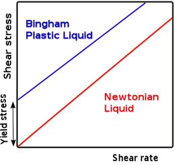
Non-Newtonian Viscosity
|
A Non-Newtonian fluid is a fluid that does not follow Newton's Law of Viscosity - the linear relation of the shear stress with the shear rate. Instead, the viscosity of non-Newtonian fluids is a function of the local shear rate or shear rate history. Many industrial and natural substances such as multi -grade motor oil, molten polymers, petroleum and blood, are non-Newtonian fluids. It is therefore important to have the capability to model non-Newtonian fluid flows. Simerics-MP provides the following non-Newtonian viscosity models:
The two models have been widely used to compute the dynamic viscosity for various types of non-Newtonian fluids. Mathematically, both the Herschel-Bulkley Model and Bingham Models have the following general relation between the shear stress ( |
 ) and the shear rate (
 ) but different model constants:
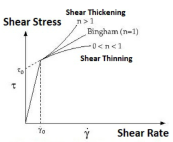

|
|

|
where

|
Critical shear rate (1/s) |

|
Consistency index |

|
Yield stress of the fluid (Pa) |

|
Power Law index. For Bingham model,  |
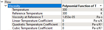
Polynomial Function of T
|
Viscosity is modelled as a function of temperature by selecting Polynomial Function of T. In Simerics-MP, viscosity is calculated based on temperature of the material, which is specified as a function of temperature with polynomial functions using three coefficients. |
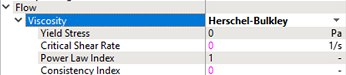
Herschel-Bulkley Model
|
The Harschel-Bulkley viscosity model in Simerics-MP, models the non-newtonian fluid in which strain experienced by the fluid is related to stress in non-linear way. Four parameters characterize this relationship, namely, Yield Stress (Pa), Critical Shear Rate, Power Law Index and Consistency Index. The Yield Stress quantifies the amount of stress that the fluid may experience before it yields and begins to flow, while the Power Law Index measures the degree to which the fluid is shear thinning or shear thickening. The Consistency Index is a constant of proportionality. |
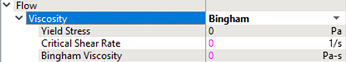
Bingham Model
|
The Bingham model requires three parameters, the Yield Stress, Critical Shear Rate and Bingham Viscosity to describe its flow.
|
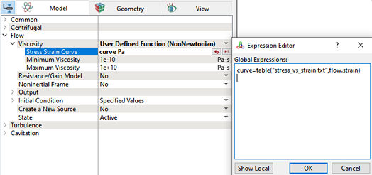
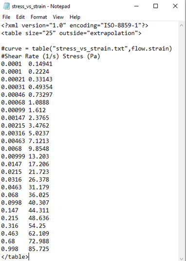
User Defined Function (Non-Newtonian)
|
Another way of computing the dynamic viscosity for Non-Newtonian fluid is by using user defined stress strain curve. In this option, user must prepare stress strain curve in table format or by polynomial equation and should be called through expression editor by accessing the variable flow.strain. The fluid strain is computed from flow.strain variable and solver takes the corresponding stress value from the table. The following example shows how to provide user defined stress strain curve. Example of using User Defined (Non-Newtonian)In this sample example, stress strain curve is provided by table format: The user can provide stress strain curve by the following steps:
|
Deformation model
The deformation model is used to model the wall compliance due to the fluid stress. It is governed by the linear theory of elasticity, on the assumption that the pipe is circular and that the wall is thin  , as follows:

|
where

|
Tension or Compression stress (Pa) |
 |
Pipe radius (m) |

|
Reference radius (m) |

|
Fluid pressure (Pa) |
|
|
Reference pressure (Pa) |

|
Wall thickness (m) |

|
Young's modulus (Pa) |

|
Poisson ratio |

The equation 5.35 is used to calculate the stresses and thereby the displacement of the wall. Simerics-MP does not physically move the grid associated with the wall to model the wall compliance. The effect of the wall motion is included by changing the effective volume of the wall cell.
Resistor Capacitor Model
The Resistor Capacitor Model is used to determine flow rate across boundaries or interfaces, with existing loads on the system. The theoretical modelling is analogous to an electrical circuit. An example of an application is the load faced by the heart in pumping blood through the arterial system. The model provides the relation between blood pressure and blood flow in the aorta or the artery.
DP-Q Curve
The DP-Q curve specifies the flow rate as a function of pressure.

|
5.36 |
where

|
Volumetric flux (m3/s) |

|
Local cell pressure (Pa) |

|
Environment pressure (Pa) |
The DP-Q curve boundary condition requires an expression or table defining the flow rate  as a function of
  for the volumetric flux input field (otherwise there is no
  dependence).
  as a function of the environment pressure and the boundary cell pressure is computed by the code and is available as a Local Expression Editor variable. The unit for
  is Pa.
Orifice
The volumetric flow is computed as if there were a circular orifice in the boundary. The equation and inputs are as follows:

|
5.37 |
where

|
Volumetric flux (m3/s) |

|
Discharge coefficient |

|
Upstream cell fluid density (kg/m3) |

|
Orifice diameter (m) |

|
“Diameter” of upstream wall surrounding the Orifice. (m) (Assumed  , such that , such that  may be ignored) may be ignored) |
Therefore, the input parameters are the discharge coefficient, orifice diameter, and ambient pressure.
Resistor
The volumetric flow across a boundary is computed based on the pressure drop and an effective resistance.
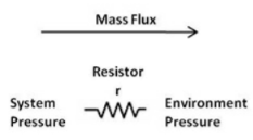
Figure 5.14 - Resistor
The equations are as follows:

|
|

|
|
where

|
Volumetric flux (m3/s) |

|
Resistor (Pa-s/m3) |
Capacitor
The volumetric flow across a boundary is computed based on the pressure drop and a capacitor of capacitance  in the system.

|
2 Elements
The flow-pressure relationship for a selected Boundary is determined based on a circuit consisting of a resistor and a capacitor. The equation for the 2 Element Resistor-Capacitor model is based on the 2-element Windkessel model 2 Broemser, Ph., et. al., ``Uber die Messung des Schlagvolumens des Herzens auf unblutigem Weg'', Zeitung für Biologie 90 (1930) 467-507. often used for heart flow modelling as shown below:

|
where

|
Volumetric flux (m3/s) |

|
Resistor (Pa-s/m3) |

|
Capacitor (m3/Pa) |
3 Elements
The flow-pressure relationship for a selected boundary is determined based on a circuit consisting of two resistors and one capacitor. The equation for the 3 Element Resistor-Capacitor model is based on the 3 - element Windkessel model often used for heart flow modelling as shown below:

|
where

|
Volumetric flux (m3/s) |

|
Resistor-1 (Pa-s/m3) |

|
Resistor-2 (Pa-s/m3) |

|
Capacitor (m3/Pa) |
Porous Media Resistance Model
Description
In many single and multiphase engineering systems, the flow domain of interest often contains irregular-shaped solid structures. The typical examples are flows through filters, perforated plates, flow distributors and packed beds. When using CFD methodology to simulate flow in such applications, the explicit treatment of the irregular-shaped boundaries is very costly, if not entirely impossible. It is therefore desirable, in many practical cases, to capture the essential features of the system and to express the flow in terms of local averaged quantities, via a porous-media approach, while sacrificing some of the details.
In Simerics-MP+, porous media has two main characteristics: porosity and flow resistance. Porosity is defined in Common module, and flow resistance is defined in Flow module. In the current version (5.1), there are two flow resistance models: Pressure Loss Model, and Darcy's Law. It is easier to use Pressure Loss Model, if flow resistance of porous media is reported as a  curve. If resistance is reported as permeability, user can directly use the value in Darcy's Law model.
For flows in porous media, the governing equations have the form:

|
5.42 |

|
5.43 |
Pressure Loss Model
Flow resistance force can be evaluated by a pressure loss model:

|
where,

|
Quadratic drag coefficient (1/m) |

|
Porosity |

|
Resistance force density (force per unit volume) (N/m3) |

|
Linear drag coefficient (Pa-s/m2) |
 |
Density (kg/m3) |

|
Velocity (m/s) |
In the solver, user needs to input  and
and  as the model parameters in porous media region.
|
Note: In most of pressure loss experiment, the porosity was not used in the test results. The velocity value used in calculation is superficial velocity, which is simply total flow rate divide by total cross-section area. Since, flow velocity is adjusted with respect to porosity in the solver, therefore the velocity in equation 5.44 is multiplied by the porosity |
 to make it consistent with the test data.
Darcy’s Law
Flow resistance force can be evaluated by Darcy's Law:

|
where,

|
Quadratic drag coefficient (1/m) |

|
Porosity |

|
Viscosity (Pa-s) |

|
Permeability (m2) |
 |
Density (kg/m3) |
Here, porosity is used for the same reason as in pressure loss model. In the solver, user needs to input Permeability and  as the model parameters in porous media region.
|
Note: The Darcy's Law (first term on the right) is based on the assumption of creeping flow through an infinitely extended uniform medium, and thus mainly applies for porous media with low flow velocities. At high velocities, however, in addition to the viscous loss, it is generally recognized that the inertial loss (the second term on the right) often plays a very important role. But generally, the source term according to Darcy's Law is calculated with an extension to the second term as shown in the above equation. |
Evaluation of Model Parameters
For many engineering problems, flow resistance of porous media are reported using  curves obtained through experiments.
where,

|
Volumetric flow rate (m3/s) |
 |
Pressure (Pa) |
A  curve can also be approximated by a 2nd order polynomial of q:

|
Where,  and
and  are two constant coefficients. Figure 5.15 gives an example of experiment
  curve together with 2nd order polynomial fitting (in MS Excel).
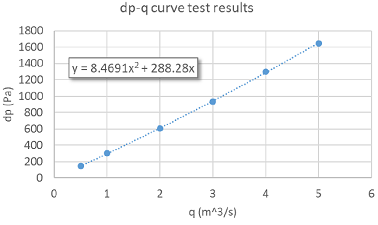
 in equation 5.44 and equation 5.45 can also be treated as
  . Where
  is the flow direction in porous media penetrating the thickness (L) of porous region. On integrating equation 5.44 and equation 5.45 with respect to
  , assuming all the properties and flow velocities are all uniform inside porous media. Also by substituting superficial velocity
  with
with  , we get:
Pressure Loss Model

|
Darcy’s Law

|
where,

|
Cross-section area of porous media (m2) |
 |
Thickness (m) |
|
Note: The pressure drops are treated as positive values in this calculation to be consistent with convention of most pressure loss measurements. |
Comparing equation 5.46, equation 5.47 and equation 5.48, we can find that:
Pressure Loss Model
 |
|
 |
Darcy’s Law

|
|
 |
By rearranging them, we get:
Pressure Loss Model
 |
|
 |
Darcy’s Law

|
|
 |
Pressure loss may be reported in  curve. Pressure Loss vs. (superficial) Velocity, as shown in Figure 5.16. And the
  curve can be approximated by a second order polynomial as in equation 5.57.
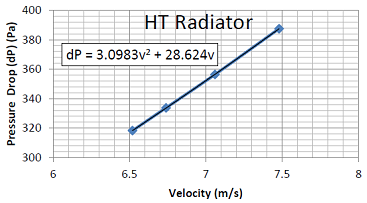

|
Similar equations can be derived to calculate flow resistance model coefficients. Substitute  with superficial Velocity V in equation 5.47 and equation 5.48, we get:
Pressure Loss Model

|
Darcy’s Law

|
Compare with equation 5.57 and by rearranging them, we get:
Pressure Loss Model
 |
|
 |
Darcy’s Law

|
|
 |
Values evaluated using equation 5.53 to equation 5.56 or equation 5.60 to equation 5.63 can be used as input parameters for porous media models. Similar equations can be derived, when pressure drop experiment data are reported in other form.
For simple porous media channels with uniform properties and uniform flow, the input parameters evaluated using the above methods can be reasonably accurate. When experiment was carried out under complicated situations, for example with highly non-uniform flow, a more accurate way to find these coefficients is from numerical experiment using Simerics-MP/Simerics-MP+. User can adjust resistance model coefficients to match experiment  relation. The initial guess can be the values from the estimation above. A recommended practice is to use pressure drop at low flowrate to calibrate linear flow resistance coefficient, and use pressure drop at high flowrate to calibrate quadratic flow resistance coefficient.
Porosity Induced Pressure Change
The value of porosity should not affect pressure loss through porous media in the current flow resistance models. However, porosity may still induce pressure change in the current simulation approach. The flow velocity inside porous media will increase with decreasing of porosity. Fluid coming from open channel to porous region needs to accelerate to a higher speed inside porous media. Similarly, when fluid exit porous media it needs to deaccelerate to a lower speed. Acceleration and de-acceleration are typically realized through pressure gradient. In both cases, pressure change can be observed close to the interface between the porous media and the open channel.