13.3 Functions
The Functions in the Expression Editor enable mathematical and logical manipulation of both Vectors and Scalars.
The functions available in Expression Editor are explained here :
- Operators
- Common to Vectors and Scalars (e.g. addition and subtraction)
- Scalars only (e.g. square roots and logs)
- Vectors only (e.g. dot and cross products)
- Logicals
- Trigonometric and Hyperbolic
- Display related functions
- Other functions
- Integration and Averaging
- Tables
13.3.1 Operators
The operators in the Expression Editor enable mathematical manipulation of both vectors and scalars. The mathematical operations available in the Expression Editor are shown in Table 13.1. In this table: a, b, c are scalars, and U, V, W are vectors.
| Expression Operators | Function | Example |
|---|---|---|
| Operators: Scalars and/or Vectors | ||
| + | Addition | a = b+c or V = U+W |
| - | Subtraction | a = b-c or V = U-W |
| * | Multiplication of two Scalars or a Scalar and a Vector | a = b*c or V = a*U (but not V = U * W) |
| Operator: Scalars Only | ||
| / | Division | a = b/c |
| exp(scalar) | Base e exponential function | a= exp(b) raises e to the power of b: a= eb |
| ln(scalar) | The natural logarithm function for e | a= ln(b) returns the natural log of b |
| sqrt(scalar) | square root function | a = sqrt(b) |
| ^ | exponential function | a= b^c raises b to the power of c: a= bc |
| Operator: Vectors Only | ||
| & | vector dot product | a = V&U (a = |V| |U| cos (angle)) |
| ^ | vector cross product | V=U^W (|V| = |U| |W| x sin (angle)  ), The
right-hand-rule is applied. ), The
right-hand-rule is applied. |
| len(vector) | returns the length of vector V | a = len(V) |
| normalize(vector) | returns a normalized unit vector V/|V| | V = normalize(U) |
| rotate(vector,angle, direction,center) | Returns a rotated vector based on the rotation angle, RHR, rotational axis and an optional rotation center. (If no center is defined, it defaults to 0,0,0) | Vrot = rotate(V,alpha,U,W) where V is the vector to be rotated, alpha is the angle in radians, and U is the axis of rotation. The right-hand-rule is applied. W is an optional center point defined as a vector. |
13.3.2 Logicals
The Logical functions in the Expression Editor enable the inclusion of logical statements. The following logical expressions are available in the Expression Editor:
| Expression Operators | Function | Example |
|---|---|---|
| true | logic true | |
| false | logic false | |
| < | less than | |
| > | greater than | |
| == | Equal in logical comparison | a = (b==3) ? 1 : 2 |
| or | logical or | |
| and | logical and | |
| ! | logical negation | !< not less than |
| a = expression ? b : c |
a = b if expression is true; a = c if expression is false |
a = (b>3) ? 1 : 2 ==> ( If b is greater than 3, a = 1 otherwise a = 2 ) |
Table 13.2 - Logicals
13.3.3 Trigonometric and Hyperbolic
The Trigonometric and Hyperbolic functions in the Expression Editor enable the inclusion of the corresponding functions in the mathematical statements. The following trigonometric and hyperbolic functions are available for scalars in the Expression Editor:
| Transcendental Expressions | Function |
|---|---|
| Trigonometric | |
| sin(radians) | sine function |
| cos(radians) | cosine function |
| cot(radians) | cotangent function |
| tan(radians) | tangent function |
| asin() | inverse sine function, returns value in rad |
| acos() | inverse cosine function, returns value in rad |
| acot() | inverse cotangent function, returns value in rad |
| atan() | inverse tangent function, returns value in rad |
| atan2(y,x ) | two variable inverse tangent function, (-pi, pi), returns value in rad |
| Hyperbolic | |
| sinh() | hyperbolic sine function |
| cosh() | hyperbolic cosine function |
| coth() | hyperbolic cotangent function |
| tanh() | hyperbolic tangent function |
| asinh() | inverse hyperbolic sine function |
| acosh() | inverse hyperbolic cosine function |
| acoth() | inverse hyperbolic cotangent function |
| atanh() | inverse hyperbolic tangent function |
Table 13.3 - Trigonometric and Hyperbolic functions
13.3.4 Display related functions
The Display related functions pertain to the Display Panel. They are used to:
- Enable rotation and/or translation of the image in the Display Panel.
- Enable the creation of a new variable with all the features of a Derived Variable, including the ability to display that function on selected Geometric Entities, such as Boundaries and Iso-surfaces.
- Variables at Points.
- Variables for XY plots.
Geometric view parameters
geom.move: (vector) translate geometry relative to Display Panel.
geom.rotate: (vector) rotate geometry relative to Display Panel. The 3 components of the vector are the same as the Z -X’-Z’’ angles defined in the View Tab in rad.
| ´ | Note: The geom functions can be activated after running the simulations. |
User defined variable for 3D display
display.varname: Defines a user variable to be used in 3D plots such as Contours / Iso Surfaces / Vectors. New variable will be added to "User Defined" under Variable in the Results Panel
#display.varname: dispname [unit]: (optional)Defines a new name with unit for a user defined display variable.
display.pref = flow.P - 101325
#display.pref: Gauge Pressure [Pa]
Upon using these expressions, the Gauge Pressure appears under User Defined Variable in the Results Panel as shown in Figure 13.5:

Variables at Monitoring Points
All the local cell variables at any monitor point can be accessed using the following format:
module[.subname].var@probe.name
Point coordinates:
probe.coord@probe_name
inletP = flow.P@probe."Point01"+101325
User defined variable for XY-Plot
plot.varname: Defines a user variable to be used in X-Y Plots. New variable will be added to Common section in the Plot Panel.
#plot.varname: dispname [unit]: (optional) Defines a new name with unit for a user defined variable.
plot.head = (flow.pt@outlet - flow.pt@inlet)/998/9.8
#plot.head: Pressure Head[m]
|
Note:
|
13.3.5 Other functions
| Expression Operators | Function | Example |
|---|---|---|
| abs(x) | absolute value function | |
| max(x,y) | maximum function | a = max(b,c) ==> a= b if b >c or a=c if c>=b |
| min(x,y) | minimum function | a = min(b,c) ==> a= b if b <c or a=c if c<=b |
| mod(x,y) | modulus function, | a = mod(c,b) ==> a = the remainder of c divided by b |
| sgn(x) | returns a flag (-1, 0, or 1) indicating the sign | a= sgn(b) ==> a = -1 if b<0 a = 0 if b=0 a = 1 if b>0 |
| step(x) | step function returns a 0 or 1 depending on the value relative to zero | a= step(b) ==> a = 0 if b<0 a = 1 if b>=0 |
Table 13.4 - Other functions
13.3.6 Integration and Averaging
The Integration and Averaging functions in the Expression Editor enable the integration of scalar or vector data on a Boundary or Volume.
integral(x, patch.name | volume.name): User defined area or volume weighted integral area or volume weighted integral in a boundary/ volume, "x" is a scalar or vector variable, or an expression of scalar or vector variables.
average(x, patch.name | volume.name): User defined area or volume average in a boundary/ volume, "x" is a scalar or vector variable, or an expression of scalar or vector variables.
Using integration and averaging functions:
# Calculating integrated and averaged data on a boundary and a volume respectively
force = integral(pre, patch.sidewall)
p_mean = average(pre, volume.port)
13.3.7 Tables
The Table functions in the Expression Editor enable the inclusion of data from external table files located in the same directory as the project file (*.spro).
The following Table functions are available in the Expression Editor:
| Table Expressions | Function |
|---|---|
| table(filename,x) | Interpolates from a 1-D Table (see Tables:1-D) |
| table(filename, x ,y) | Interpolates from a 2-D Table (see Tables:2-D) |
| table(filename, vector) | 3-D Mapping table format (see Tables:3-D). It can be any vector, most commonly used as coordinate vector. Considers exact point data and no interpolation from the table |
Table 13.5 - Table functions
# Extracting information from tables
p = table("inlet_pressure.txt",time)
density = table("R134a_density.txt",temp,pre)
Table Format: 1-D
The 1-D Table function table(filename,x) enables access to a 1-D data table located in the same directory as the project file (*.spro).
Format of the 1-D Table for Uniform Distribution :
<?xml version="1.0" encoding="ISO-8859-1"?>
<table size="n" min="xmin" max="xmax" outside="flat | extrapolation">
# comment - values (x is assumed to have uniform distribution with xmin and xmax as bounds and n values in between)
v1
v2
…
vn
</table>

Format of the 1-D Table for Non-Uniform Distribution is :
<?xml version="1.0" encoding="ISO-8859-1"?>
<table size="n" outside="flat | extrapolation">
# comment - values (x is assumed to have non-uniform distribution)
x1 v1
x2 v2
…
xn vn
</table>

In the table syntax, outside = “flat” or outside = "extrapolation"under the table tag dictates how to determine a value when the input x, y is out of the range. "flat" denotes that the value of the closest bound is considered, and "extrapolation" denotes that the values are extrapolated from the nearest bound values.
|
Note: Comments can be input by placing a hash-mark “#” in front of the text. They are not inserted before the xml line (line 1). |
Table Format: 2-D
The 2-D Table function table (filename,x) enables access to a 2-D data table located in the same directory as the project file (*.spro). 2D tables are used to specify variables which depend on two other independent variables.
Format of the 2-D Table for Uniform Distribution :
<?xml version="1.0" encoding="ISO-8859-1"?>
<table size="nx my" min="xmin ymin" max="xmax ymax" outside="flat | extrapolation">
# values (x and y assumed to have uniform distribution)
v(x1,y1) v(x2,y1) … v(xn,y1)
v(x1,y2) v(x2,y2) … v(xn,y2)
…
v(x1,ym) v(x2,ym) … v(xn,ym)
</table>

Format of the 2-D Table for Non- Uniform Distribution :
In the format outside = “flat” or outside = "extrapolation"under the table tag dictates how to determine a value when the input x, y is out of the range.
<?xml version="1.0" encoding="ISO-8859-1"?>
<table size="nx my" outside ="flat | extrapolation">
# x and y variable ranges
x1 x2 … xn
y1 y2 … ym
# values table
v(x1,y1) v(x2,y1) … v(xn,y1)
v(x1,y2) v(x2,y2) … v(xn,y2)
…
v(x1,ym) v(x2,ym) … v(xn,ym)
</table>

In the table syntax, outside = “flat” or outside = "extrapolation"under the table tag dictates how to determine a value when the input x, y is out of the range. "flat" denotes that the value of the closest bound is considered, and "extrapolation" denotes that the values are extrapolated from the nearest bound values.
|
Note: Comments can be input by placing a hash-mark “#” in front of the text. They are not before the xml line (line 1). |
Table Format: 3-D
The 3-D Table function table (filename,vector) enables access to a 3-D data table located in the same directory as the project file (*.spro). The 3-D tables are used to specify a variable distribution over a boundary/volume.
Format of the 3-D Table :
<?xml version="1.0" encoding="ISO-8859-1"?>
<table mapped_size="n" allowed_error="1" outside_valve="minimum">
# comment - values (x is assumed to have uniform distribution with xmin and xmax as bounds and n values in between)
x1 y1 z1 v1
x2 y2 z2 v2
…
Xn yn zn vn
</table>
In the table syntax,
- The table mapped size denotes the number of mapped points.
- The allowed_error of ”1” maps the specified values within a tolerance of 1 m on the boundary. The distance to the closest point (can be find in the table) has to be less than this allowed error. If the distance is larger than this allowed error, then it is assumed that the point is outside.
- outside_value can be “minimum” or “maximum, these dictates how to determine a value when the input is out of the range "minimum" or “maximum” denotes that the lowest\highest value in the table are considered.
# Extracting data from tables,
T_fluid = table("solid_temperature.txt", coord);
Mapping variables using tables
User can specify a variable distribution over a boundary/volume using a table. This is done using the X,Y,Z coordinates specifying the distribution of the variable in form of a table at that respective Geometric Entity, such as a Boundary or a Volume. This is primarily used for:
- Specifying input on an entity from test data or external software in the form of 3D coordinates.
- Mapping of boundary conditions for fluid-solid coupled simulations (eg. Heat flux/Temperature distribution on a boundary).
- Specifying initial conditions for Volumes/Boundaries to start a simulation.
- Specifying properties (eg. Density, Conductivity) as conditions on an entity, such as Volume.
-
Mapping velocity vector
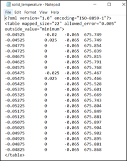
Figure 13.10 shows an example of a table specifying temperature distribution over a boundary. The temperature specified in the table is mapped to the respective coordinates. The first 3 columns correspond to the X, Y, Z coordinates and the 4th column shows the temperature at each of those coordinates points.

Figure 13.10 - Table for Temperature Distribution on Boundary
The table as shown in Figure 13.10 is read at the appropriate boundary, to specify the distribution as the Specified Temperature boundary condition.
Similarly, tables can also be used to specify the distribution of other variables such as pressure, heat flux etc. as boundary conditions.
Mapping of temperature is a typical requirement for an e-motor application (loosely coupled CHT simulation). Here, temperature on a required boundary is obtained from solid simulation and mapped to fluid boundary during fluid simulation. Follow the below steps to map temperature distribution on a boundary.
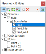
- Select required boundary in the Geometric Entities Panel as shown in Figure 13.11.
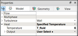
- Select Specified Temperature under Heat list in the Properties Panel as shown in Figure 13.12.
- Enter T_fluid K for Temperature.
- Call the text file using expression editor in Tables format, as shown in Figure 13.13. Here, text file solid_temperature.text is obtained from solid simulation.
-
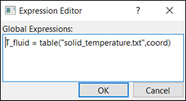
Click Edit Expressions
 icon next to T_fluid and enter T_fluid = table("solid_temperature.txt",coord) under Global Expressions as shown in Figure 13.14.
 - Click OK, to close the Expression Editor dialog box.