Wall Physics
Turbulent flows are significantly affected by the presence of walls. In wall-bounded flows, first and foremost, the mean velocity field is affected by the physical constraint of the flow-wall non-slip condition. For turbulent flows, the turbulence is also altered by wall boundaries. In the region very close to the wall, viscous damping reduces the tangential velocity fluctuations, while kinematic blocking decreases the normal fluctuations. Towards the outer layer of the near-wall region, the turbulence is rapidly augmented due to the large gradients of the mean velocity. To successfully predict wall-bounded turbulent flows, it is essential to accurately represent the near-wall effects on turbulence.
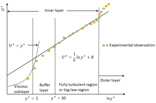
In near-wall modelling, the region close to the wall is typically subdivided into three layers based on a non-dimensional normal-to-wall distance,  . In the innermost layer,
  , the so-called “viscous sublayer”, the flow is almost laminar, and the (molecular) viscosity plays a dominant role in momentum, heat and mass transfer. In the outer layer,
  , commonly called the inertial layer or fully-turbulent region, turbulence plays a dominant role. Finally, there is an interim region between the viscous sublayer and the fully turbulent layer (buffer layer),
  , where the effects of molecular viscosity and turbulence are equally important. While near-wall turbulence/low-Re number turbulence models could resolve all the three wall sublayers, they usually require very fine near-wall meshes, say, a prerequisite for the near-wall cell,
  typically less than 1. Often, an economical alternative, the wall functions, have been used to account for the wall effect. In this approach, the viscosity-affected inner region (viscous sublayer and buffer layer) is not resolved. Instead, semi-empirical formulae called “wall functions” are used to bridge the viscosity-affected region between the wall and the fully turbulent core. As a result, the near-wall mesh requirement is significantly lessened. In fact, the value of
  at the near-wall cell should be in the fully turbulent outer layer, usually between 30 and 60.
|
Figure 5.54 - Near wall region characteristics |
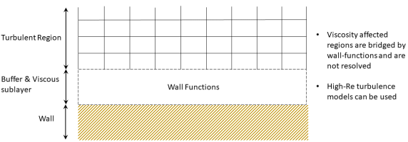
Figure 5.55 - Wall function treatment |
 :
:  and
and  where
where  is the friction velocity
Simerics-MP offers the wall function approach for near-wall modelling, consistent with the high-Re numbers of the standard and  turbulence models, as described in the previous section.
Standard Wall Function
The standard wall function serves not only as the most widely-used near-wall treatment, but also the basis for the development of more advanced near-wall models, including the more elaborate wall functions. The wall functions consist of the law-of-the-wall for the mean velocity, temperature and species, and the formulae for the near-wall turbulent quantities. The specific formulations are listed as follows:
Momentum:
The law-of-the-wall for mean velocity defines the relationship between the dimensionless mean velocity  and non-dimensional wall-to-cell distance
  :
:
|
|

And over a near-wall cell " ", the wall variables are defined or calculated as follows:
Wall shear stress:
|
|

Wall friction velocity:
|
|

Dimensionless mean velocity:
|
|

Dimensionless distance from wall:
|
|

where

|
Von Karman constant = 0.41 |

|
Empirical constant = 9.54 |

|
Tangential velocity component at the wall-adjacent cell, P; (m/s) |

|
Turbulence kinetic energy at the wall-adjacent cell, P; (m2/s2) |

|
Distance from the wall-adjacent cell to wall; (m) |

|
Dynamic viscosity of the fluid; (Pa-s) |

|
Fluid density (kg/m3) |

|
Wall shear stress (Pa) |

|
Empirical constant = 0.09 |
Energy:
Following Reynolds’ analogy, the law-of-the-wall for the temperature is assumed to be similar to the law-of-the-wall for the mean velocity: the logarithmic law applies for the mean temperature, and the thickness of the thermal conduction layer ( ) can be estimated using the momentum sublayer thickness (
 ) and the Prandtl number (
 ):
):
|
|

where  and
and  are the heat capacity and heat conductivity of fluid, respectively.
For turbulent flows, there are two diffusion terms in the averaged energy equation: effective thermal conductivity (the first term on the right-hand side) and viscous-heating (the second term):
|
|

where  is effective heat conductivity. In the standard
  model,
  ; while for the
  model,
  , and
, and  is calculated from equation 5.104.
Clearly, the wall treatment needs to consider both diffusion terms. In the standard wall function, the non-dimensional temperature for wall scaling is thus defined as:
|
|

where  ̇ is wall heat flux;
  is the wall temperature. The non-dimensional convective-conductive term
  , and the viscous heating term
  (usually only included in compressible flows in pressure-based solvers) are as follows:
|
|
|
|
|


where  is computed with the formulation given by Jayatilleka1C. Jayatillaka, "The Influence of Prandtl Number and Surface Roughness on the Resistance of the Laminar Sublayer to Momentum and Heat Transfer", Prog. Heat Mass Transfer, 1.193-321, 1969.
|
|

And  is the turbulent Prandtl number = 0.85);
  is the mean velocity at
  ; and
; and  is the non-dimensional thermal sublayer thickness. Numerically, it is defined as the
  value at the intersection point between the linear law and the logarithmic law in equation 5.116. It can be obtained using Newton’s iterative method:
|
|
|
|
|


At the intersection,  , and
, and  . From Newton’s iterative method, we have:
|
|

with the initial value of  .
.
Species
With wall functions, the species transport is assumed to behave analogously to heat transfer. Similar to equation 5.116, for constant property flows with no viscous dissipation the law-of-the-wall for species-i can be expressed as:
|
|

where  are wall, local and non-dimensional mass fraction of species-i, respectively;
  is the diffusion flux of species-i on the wall;
  and
and  are the molecular and turbulent Schmidt numbers; and
  and
and  are estimated in a similar way to
  and
and  , with Schmidt numbers to replace the Prandtl numbers.
Turbulence
In the  models with the standard wall functions, the boundary conditions are:
k-equation: Zero-flux/zero-gradient (wall value:  )
)
|
|

ε-equation: Fixed value obtained from local equilibrium assumption in the wall function
|
|

Based on the wall function hypothesis of constant turbulent wall shear in the logarithmic region, the production term  is corrected as follows:
|
|

And from equation 5.124 and equation 5.125, the dissipation rate is
|
|

The  value on the wall surface (face),
 , is extrapolated as
|
|

Non-Equilibrium Wall Function
The standard wall function approach gives reasonable predictions for many high-Reynolds number wall-bounded flows. However, when modelling pressure-driven, rapid-changing flow phenomena such as separation, reattachment and impingement, it is highly desirable to account for the effects of pressure gradients on flow and turbulence in the law-of-the-wall, in particular, in the prediction of wall shear and heat transfer.
Based on the standard wall function, Kim and Choudhury2S.-E. Kim and D. Choudhury, "A Near-Wall Treatment Using Wall Functions Sensitized to Pressure Gradient", In ASME FED Vol. 217, Separated and Complex Flows, ASME, 1995 proposed a two-layer-based, non-equilibrium wall function to partly account for the effects of pressure gradients. In this approach, modifications have been introduced to the law-of-the-wall for the mean velocity and the wall turbulence quantities, while the law-of-the-wall mean temperature or species mass fraction remains the same as in the standard wall function described above. The detailed formulations are described in the following:
Momentum
To include the effect of pressure gradients, a modified dimensionless mean velocity,  , is introduced in the law-of-the-wall for mean velocity:
|
|

And the wall variables are calculated by the following expressions:
Dimensionless mean velocity:
|
|

Dimensionless distance from wall:
|
|

Modified mean velocity:
|
|

Physical thickness of viscous sublayer:
|
|

where  is the near-wall cell pressure gradient tangent to the wall,
 and
and  .
.
Turbulence
The non-equilibrium wall function accounts for the effect of pressure gradients on the distortion of the mean velocity profiles. In such cases the assumption of local equilibrium, the production of the turbulent kinetic energy is equal to the rate of its destruction, is no longer valid. To determine the near-wall cell turbulence production term  and dissipate rate
  , a two-layer concept has thus been introduced to characterize the wall-adjacent cells. Specifically, it assumes that the near-wall cells consist of a viscous sublayer and a fully turbulent layer, and the turbulence quantities have the following profiles:
Turbulent shear stress:
|
|

Turbulent kinetic energy:
|
|

Rate of turbulent dissipation:
|
|

And the turbulence production term  and dissipate rate
  are the volume-averaged values over the near-wall control volume
  :
:
|
|
|
|
|


where  is the volume of cell
  .
.
equation 5.136 and equation 5.137 clearly indicate that the near-wall turbulence depends on the local proportion of the viscous sublayer and the fully turbulent layer over the control volume  . In highly non-equilibrium flows, it could vary greatly from one cell to the other. Therefore, this wall function approach, in effect, partly accounts for the non-equilibrium effects that are neglected in the standard wall functions.
Unified Wall Function
As discussed above, both the standard and non-equilibrium wall-functions can only be applied for the inertial (fully turbulent) layer since the viscosity-affected inner region (viscous sublayer and buffer layer) is not resolved. As a result, the limitation imposes a restriction on the near-wall mesh, ideally satisfying the condition,  , to avoid unbounded errors in wall shear stress, heat and mass transfer with too small
  . Obviously, it is inconvenient for grid generation and/or mesh refinement, in particular, for complex geometries in industrial applications.
To overcome such a deficit, Shih et al 3Shih, T.-H., Povinelli, L.A., and Liu, N.-S., “Application of Generalized Wall Function for Complex Turbulent Flows”, J. of Turbulence, 4 (2003) 015. proposed a unified wall function, which is applicable for the entire near-wall layer covering the viscous sublayer, buffer layer and inertial (fully-turbulent) sublayer. In this approach, by examining the asymptotic solutions for zero pressure gradients and zero wall shears, Shih et al derived a general asymptotic solution for both inertial and viscous sublayers. To model the buffer layer, a unified law-of-the-wall formulation is then obtained based on the asymptotic solutions and fitting functions.
Fully-Turbulent Sublayer
In addition to the wall friction velocity,  , to account for wall shears, a pressure gradient velocity,
  , is introduced to characterize the effect of wall pressure gradients. The definitions are given below:
Wall frictional velocity:
|
|

Wall pressure gradient velocity:
|
|

where  is the fluid kinematic viscosity; and
  is the magnitude of the tangential wall pressure gradient
In a wall bounded flow, there are asymptotic solutions for both zero wall pressure gradient and zero wall shear boundary layers, respectively:
Zero pressure gradients (Millikan4Millikan, C.B.A., 1938, "A critical discussion of turbulent flows in channels and circular tubes”, Pages 386-369 of: Proceedings of the Fifth International Congress of Applied Mechanics.):
|
|

Zero Wall Shears (Tennekes and Lumley5Tennekes H and Lumley J L 1972 A First Course in Turbulence (Cambridge, MA: MIT Press)):
|
|

where the constants are  ,
,  ,
,  and
and  .
.
To generalize the law-of-the-wall formulation, Shih et al introduced a hybrid velocity scale:
|
|

And the tangential mean flow velocity is
|
|

With the substitution of equation 5.140and equation 5.141 into equation 5.143 and the division of  by
by  , the generalized asymptotic solution can be obtained in the fully turbulent sublayer:
|
|

where
|
|

This generalized wall function is valid for both zero-wall-shear-stress and zero-wall-pressure-gradient turbulent boundary layers. In fact, equation 5.144 would exactly return to equation 5.140 for flows with zero pressure gradient, and equation 5.141 for flows with zero wall shear stress. Therefore, this generalized wall function can be applied to wall bounded complex flows with acceleration, deceleration and recirculation.
Viscous Sublayer
In the viscous sublayer, the turbulent stresses are negligible, and the flow characteristic is predominately laminar. The generalized wall function has the form:
|
|

Unified Wall Function
The buffer layer, , is between the viscous sublayer and fully-turbulent layer. In this region, the viscous and turbulent stresses are equally important. Unlike the other two sublayers, no theoretical asymptotic solution can be obtained. However, following the approach originated by Spalding6Spalding, D.B., 1961, "A single formula for the law of the wall." Transactions ofth ASIDE, Series E: Journal of Applied Mechanics, 28,455-458. (who did not consider the effect of pressure gradient), Shih et al introduced a new turbulent stress model for the buffer region. Combining the generalized wall functions, equation 5.144 and equation 5.146, Shih et al developed a single analytic function, the unified wall function, for the entire near-wall layer covering the viscous sublayer, buffer layer and inertial (fully-turbulent) sublayer.
Introducing two dimensionless cell-to-wall distances based on the wall shear velocity ( ) and wall pressure gradient velocity (
 ), respectively:
|
|
|
|
|


one can combine equation 5.144 and equation 5.146 to form a single unified law-of-the-wall formulation:
|
|

where
|
|
|
|
|


And the first term represents the law-of-the-wall at zero pressure gradient (standard wall function), while the second one is the law-of-the-wall for zero wall shear stress (effect of pressure gradients).
Further, to expand equation 5.149 and include the buffer layer, Shih et al gave the following piecewise fitting functions to define  :
:
|
|
|
|
|


And the coefficients for equation 5.152 and equation 5.153 are listed in the Table 5.12 and Table 5.13 respectively:

|

|

|
||
|---|---|---|---|---|
| 1.0 | 1.0E-02 | -2.9E-03 | ||

|

|

|

|

|
| -0.872 | 1.465 | -7.02E-02 | 1.66E-03 | -1.495E-05 |

|

|

|

|

|
| 8.6 | 0.1864 | -2.006E-03 | 1.144E-05 | -2.551E-08 |
 , Shih et al

|

|
|||
|---|---|---|---|---|
| 0.5 | -7.31E-03 | |||

|

|

|

|

|
| -15.138 | 8.4688 | -0.81976 | 3.7292E-02 | -6.3866E-04 |

|

|

|

|

|
| 11.925 | 0.93400 | -2.7805E-02 | 4.6262E-04 | -3.1442E-06 |
 , Shih et al
 With the unified wall function, the wall shear stress is obtained from equation 5.149:
|
|

And the production term in the adjacent wall cell is corrected as follows:
|
|

Rough Wall Model
The laws of the wall discussed above are appropriate only when wall surfaces are considered to be hydraulically smooth. A non-smooth/rough wall can have a significant effect on turbulent flows, where the wall roughness typically leads to an increase in turbulence production. This can in turn result in significant increase in the wall shear stress and heat transfer coefficients. To accurately predict near-wall flows, it is therefore important to include the effects of wall roughness in the law-of-the-wall formulation.
Experiments in roughened pipes and channels indicate that wall roughness increases the wall shear stress and breaks up the viscous sublayer in turbulent flows. Compared to the smooth wall, it has established that the mean velocity profile near a rough wall, in the standard  formulation, has the same slope (
 ) but a different intercept (downward shift):

|
where  depends, in general, on the type and size of the roughness, and no universal function is valid for all types of roughness. For sand-grain roughness, however,
  has been found to be well-correlated with the non-dimensional roughness height, which is defined as:

|
where h is the physical roughness height. And the shift  can be expressed as:

|
It may be noted that when  , it is considered to be a hydraulically smooth wall.
Figure 5.56 shows Simerics' wall roughness predictions compared with rough wall pipe flow data. Here  is the roughness height(m) and the constant
  , where
  is the wall shear stress as shown in equation 5.109.
  is the density and
  is the mean velocity.
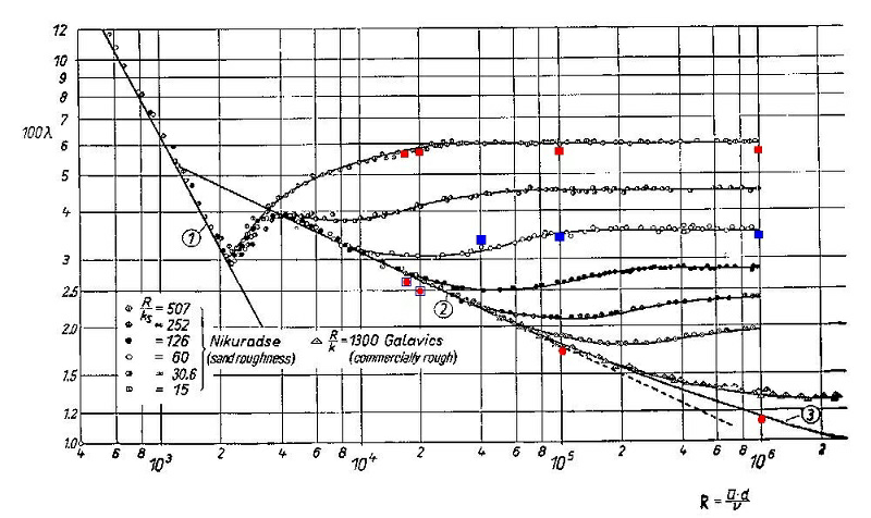
Figure 5.56 - Simerics' wall roughness predictions (colored points) compared with rough wall pipe flow data from Schlichting, Boundary Layer Theory, 6th Edition, 1968 ISBN 07-055329-7 pg. 580