You are here: Physics Modules > Flow > Output Variables

5.2.4 Output Variables

This section explains the outputs that are obtained from the Flow module. They are categorized as follows:

• Primary Variables

• Property Variables

• Derived Variables

• Integrated Quantities
• Pressure Distribution
• Velocity Distribution
• Cycle Pressure Distribution

Note: In order to display the contours and X-Y plots, or to write the outputs into an ascii file, the outputs on each Geometric entity (such as Boundary, Volume, Interface or Points) need to be activated in the Model Tab of the Properties Panel.

Primary Variables

Primary Variables are the fundamental variables that characterize the physical process in the module. They are usually obtained by directly solving transport equations or through physical constitutions. The primary variables can be displayed in the GUI Viewing Window for selected Geometric Entities as well as written to the ascii file Filename_points.txt. They can also be viewed as X-Y Plots for Point Probes.

For the Flow module, a list of Primary Variables is shown in the table below:

Primary Variables are automatically activated for selected Geometric Entities, including Boundaries, Derived Surfaces, Interfaces, Streamline, Particles and/or Volumes, depending on the modules selected.

 

Property Variables

Property Variables are the physical properties for the fluid(s) and solid(s) in the domain. They are required as a part of the solution. They may be displayed in the GUI Viewing Window for selected Geometric Entities as well as written to the ascii file Filename_points.txt (when activated). They can also be viewed as X-Y Plots for Point Probes.

For the Flow module, a list of Property Variables is shown in the table below:

As shown in Figure 5.46, Property Variables are automatically activated for output on selected Geometric Entities, including Boundaries, Derived Surfaces, Interfaces, Streamline, Particles and/or Volumes, depending on the modules selected. For Point Probes, however, explicit activation is required.

 

 

 

 

Figure 5.46 - Output activation for points-Property variables

 

Derived Variables

Derived Variables are engineering data computed from the Primary Variables. While not required as a part of the solution, they provide valuable information for analysis of the results. They can be displayed in the GUI Viewing Window for selected Geometric Entities as well as written to the ascii file Filename_points.txt (when activated). They can also be viewed as X-Y Plots for Point Probes.

A list of the Derived Variables for the Flow module is shown below:

As shown in Figure 5.47, Derived Variables are automatically activated for output on selected Geometric Entities, including Boundaries, Derived Surfaces, Interfaces and/or Volumes, depending on the modules selected. For Point Probes, however, explicit activation is required.

 

 

 

 

Figure 5.47 - Output activation for Points-Derived Variables

Integrated Quantities

An Integrated Output is the averaged or total value of a variable over a Boundary, Interface or Volume. When available and activated, the integrated quantities can be stored in the ascii file Filename_integrals.txt as well as be displayed in the GUI using X-Y Plots.

To access the variables listed below using expressions, the syntax given under Expressions column in Table 5.8 is used with a suffix “@boundary or volume name” such as pressure_outlet = flow.p@outlet.

A table of the Integrated Quantities for the Flow module is shown below:

When a pump template is used, user can access Revolution averaged quantities at the boundaries using the following syntax:

pumptype.[variable]@patch

pumptype could be centrifugal, gerotor, gear etc.,

For a selected Geometric entity, the integrated outputs must be explicitly activated as shown in Figure 5.48.

 

 

 

 

Figure 5.48 - Output activation-Integrated quantities

Note: When a boundary is modelled as a flexible wall by specifying Wall Type as Flexible, the variables Wall Displacement (m) and Wall Velocity (m/s) are available for output in theGUI Display Window under Boundary Variables.

 

Pressure Distribution

The Pressure Distribution output is activated for a selected boundary under the Flow module as follows:

• Geometric Entities Panel > Boundaries > [Desired Boundary]
• Properties Panel > Model Tab > Flow > Output > User Select > Pressure Distribution > Yes

The Pressure Distribution for selected boundaries is output in a separate file: Filename_boundary_pressure.txt.

The Pressure Distribution is output at the same frequency as the result files are saved. It is available for Wall and Rotating Wall Boundaries. In addition, Pressure Points Connectivity between points may also be output in Filename_boundary_connections.txt.

 

Note: Pressure Distribution is available as output for Wall and Rotating Wall and other solid boundaries (such as Conjugate Wall Interfaces). Pressure Distribution output on boundaries can be used to specify a force input for structural simulations to predict deformation, fatigue etc.

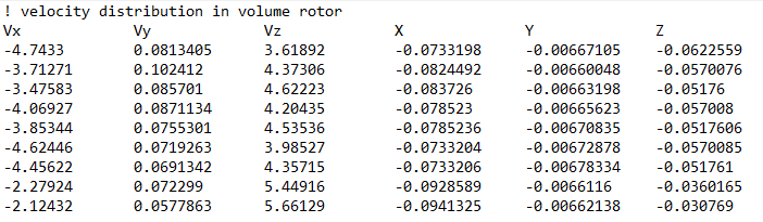
Velocity Distribution

The Velocity Distribution output is activated for a selected volume under the Flow module as follows:

• Geometric Entities Panel > Volumes > [Desired Volume]
• Properties Panel > Model Tab > Flow > Output > User Select > Velocity Distribution > Yes

The Velocity Distribution for selected volumes is output in a separate file: Filename_volume_velocity.txt as shown in Figure 5.50

The Velocity Distribution is output at the same frequency as the result files are saved.

 

Cycle Pressure Distribution (Avg/Min/Max)

The Cycle Pressure Distribution outputs are spatial distributions of "Time Average", "Time Minimum" or "Time Maximum" values of pressure on Wall or Rotating Wall boundaries:

• "Time Average" is the average values during a "Period" of time.

• "Time Minimum" is the minimum values encountered during a "Period" of time.

• "Time Maximum" is the maximum values encountered during a "Period" of time.

The "Period" is defined as number of time steps of a transient simulation. This “Period” is specified by the Cycle Computation Interval. The Cycle Pressure Distribution output is activated for a selected boundary, as follows:

• Click Common in the Model Panel.
• In Properties Panel > Model Tab, set Cycle Computation Interval, which is the number of time steps for the "Period" user wants to calculate time average, or find minimum and maximum values.
• Select Geometric Entities Panel > Boundaries > [Desired Boundary].
• Select Properties Panel > Model Tab > Flow > Output > User Select > Cycle Pressure Dist. (Avg/Min/Max) > Yes.

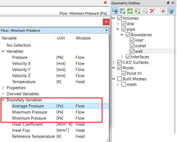
The added outputs are shown in the Results Panel under Variable > Boundary Variables as shown in Figure 5.52. They are plotted as contours on the selected boundary. The Cycle Pressure Distribution output is available for Wall and Rotating Wall Boundaries.

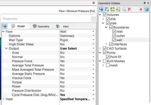
Figure 5.51 - Cycle Pressure Distribution Boundary condition

Figure 5.52 - Results Display

Note: Cycle Pressure Distribution is available as output for Wall and Rotating Wall and other solid boundaries (such as Conjugate Wall Interfaces). Users are recommended to turn on the time average/maximum/minimum output at the very beginning of simulation for all the variables of interest, and use the physical period (i.e. time step for one Pump pocket rotation or a complete revolution) as the “Period” whenever possible.