Modelling of Radiative Heat Transfer

In a thermal fluid system, the solid surfaces and/or the fluid flow may be subjected to heating or cooling due to radiation. In CFD models, the radiative heat transfer is accounted for by solving the Radiative Transport Equation (RTE) and then obtaining the radiative source term for the total energy conservation equation. Given the complex nature of thermal radiation (described in the previous section), however, numerical modelling of radiation is a daunting and time-consuming task. For practical applications, therefore, instead of attempting solutions for the radiative transport equation over space (position and direction) and time for all wavelengths, several radiation models are developed to obtain realistic solutions for different applications yet with manageable computational time and cost. Specifically, one of the widely used modelling approaches, Surface-to-Surface (S2S) radiation model, has been the chosen model in Simerics-MP. In this section, hence, special focus will be directed at this S2S model, while the radiative transport equation and a brief overview of the radiation models will also be presented.

Radiative Transfer Equation

As a ray of radiation traverses a layer of an absorbing, emitting, and scattering medium in a particular direction, it can lose energy through both absorption and scattering away from the ray, and gain energy from light sources in the medium through emission and the scattering directed towards the ray. The overall energy balance of the ray over an infinite layer of the medium results in a differential equation, which is commonly known as the radiative transport equation (RTE).

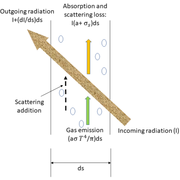
Figure 5.167 - Radiative Heat Transfer

To derive the radiative transport equation, one may consider that an incoming ray of radiation with the intensity of travels across a medium (for example, a gas) with the incremental thickness in the direction of , as shown in Figure 5.167. Through the medium layer, the incidence at the location and direction is changed in four ways acting to either increase (energy gained +) or decrease (energy lost -) the radiation intensity :

Absorption: The medium (gas in the example) absorbs a fraction of the radiation traversing it. With the absorption coefficient , the radiation energy lost through absorption is:

5.410

Scattering: The medium (gas) scatters a fraction of the radiation energy to another direction (away from direction ) when the ray traverses the medium. With the scattering coefficient , the radiation energy lost through scattering is:

5.411

Emission: The medium emits radiation energy to the ray as a gray-body according to its local temperature () and emission characteristics to the ray. From the Stefan-Boltzmann’s law and the reciprocity between emission and absorption, equation 5.402 and equation 5.407, the radiance emitted by the medium is: .

Further, assuming that n is the refractive index of the medium (defined as the ratio of the velocity of light in vacuum to its velocity in the specified medium), the actual energy gained by the ray of radiation is:

5.412

Scattering of Other Radiation: A fraction of other radiation sources existing in the layer of the medium is scattered into the ray of radiation dependent on the position and direction vectors and . Introducing to represent the direction and solid angle of the radiation beam, and to be the phase function, we have then the fraction of intensity of a ray traveling in all directions to be scattered to the direction of as:

5.413

Note that in equation 5.413, the scattering processes are ignored.

With the incoming radiation,, and the outgoing radiation, , the radiative energy balance in the direction has the form:

5.414

Substituting equation 5.410 to equation 5.413 into equation 5.414, and dividing it by , we have the radiative transport equation (RTE) as follows:

5.415

The RTE is a first order integro-differential equation for the radiation intensity in a fixed direction, . To solve this equation within a domain, in addition to the temperature field within the domain, boundary conditions for are also required on both the internal and external surfaces, and the interfaces between two different media.

As for the local medium temperature, it is obtained by solving the total energy (including the radiative sources) conservation equation, described in the Heat module. For the thermal radiation, however, the boundary treatment is quite complex and depends on the radiation models. In general, a boundary can be an opaque (emitting, reflecting and absorbing), or a semi-transparent medium (also transmitting). Furthermore, reflection and transmission can be diffuse and/or specular. For example, on an emitting and reflecting opaque boundary with gray radiation, depending on the type of reflection, the intensity of a ray can be expressed in the following:

Opaque Boundary with Diffuse Emission and Reflection:

5.416

Opaque Boundary with Diffuse Emission and Specular Reflection:

5.417

where is the normal-to-surface unit vector at position ; and are the direction and solid angle of a diffusely reflected ray (uniform reflection in all directions); is the direction of the specularly reflected ray (perfect reflection depending on the incidence); and are the surface reflectivity, diffuse reflectivity and specular reflectivity, respectively, which have the following relationship:

5.418

With given boundary conditions, equation 5.415 governs the transport of the radiation intensity in a specified direction. For gray radiations, equation 5.415 should be solved in all the different directions within a sphere. For non-gray radiations, the intensity depends also on the wavelengths. Therefore, it needs to be solved in all directions over the entire spectrum of the wavelengths. Clearly, the direct solution of the radiative transfer equation is very time consuming. In many engineering simulations, therefore, it is desirable to use somewhat simplified yet approximate models to account for the directional and spectral dependencies. In CFD simulations, the following radiation models are routinely adopted, in which the detailed description may be found in references 1R. Siegel and J. R. Howell, “Thermal Radiation Heat Transfer”, Hemisphere Publishing Corporation, Washington DC, 1992. .

Each model has its own advantages and limitations regarding accuracy and cost. For example, the Rosseland model does not solve a transport equation for the incident radiation. It is the fastest radiation model and requires the least extra memory. But it can be only used for optically thick (optical thickness is the natural logarithm of the ratio of incident to transmitted radiant power in a medium) media due to its overly simplification of the radiative transport equation. On the other end, the discrete ordinates (DO) radiation model transforms equation 5.415 into a transport equation for radiation intensity in the spatial coordinates {} and solves it over a finite number of discrete solid angles associated with the vector direction . The number of the solid angles selected directly determines the accuracy and the computational cost. The DO modelling approach is also identical to that used for the fluid flow and energy equations. At present, it is the most general radiation model that spans the entire range of optical thicknesses and can be applied to problems ranging from surface-to-surface radiation to participating radiation such as a combustion system. However, the computational cost of DO model is still substantially high, in particularly for non-gray radiations.

Among the above-mentioned radiation models, the surface-to-surface (S2S) radiation model is particularly good for modelling the enclosure radiative transfer without the consideration of the participating media. The typical examples are the radiative space heaters, and automotive underhood/underbody systems. In those situations, the radiation models for participating radiation may not always be efficient. As compared to the DO radiation model, the S2S model has a much faster time per iteration, though the view factor calculation itself can be CPU-intensive. In Simerics-MP, the current choice of model for radiative heat transfer is the S2S radiation model.

Surface-to-Surface (S2S) Radiation Model

The surface-to-surface radiation model accounts for the radiation exchange in an enclosure of gray-diffuse surfaces without participating media. The surface-to-surface radiative energy exchange depends on two main factors: the radiative characteristics of the involved surfaces, and the geometrical parameters including the surface areas and shapes, and the relative position to reach other (separation distance and orientation). In the S2S radiation model, the surface radiative heat transfer is considered by the gray-diffuse radiation model, while the geometrical parameters are accounted for by a geometric function called "view factor".

Gray-Diffuse Radiation

The S2S radiation model assumes that the surfaces are gray and diffuse (gray radiation). With a gray surface, both emissivity () and absorptivity () of the surfaces are independent of the wavelength of the outgoing and incoming rays. According to the Kirchhoff’s law of thermal radiation, indicated in equation 5.402, the emissivity equals the absorptivity:

5.419

Furthermore, with the assumption of a diffuse surface, no specular reflection occurs on the surface and the reflectivity () of incident radiation at the surface is isotropic with respect to the solid angle. From equation 5.418, we have the surface reflectivity as:

5.420

where and are the surface specular and diffuse reflectivity, respectively.

For a non-opaque or a semi-transparent surface, the transmissivity (), is also independent of the wavelengths:

5.421

The gray-diffuse surface-to-surface model has, for practical interests, the fundamental assumption that the exchange of radiative energy between surfaces is virtually unaffected by the medium that separates them. Thus, if a certain amount of radiant energy () is incident on a surface per unit area (Irradiance), the portions of the radiative energy reflected, absorbed and transmitted are , and respectively. Since for most applications, the surfaces in question are opaque to thermal radiation in the infrared spectrum, the radiative surfaces can be further considered as opaque. The transmissivity, therefore, can be neglected (). From equation 5.401 and equation 5.402, the surface reflectivity is then expressed as:

5.422

with the assumptions of the surface gray-diffuse radiation, the S2S modelling equation will be constructed based on energy conservation on each surface.

S2S Modelling Equation

The main assumption of the S2S model is that in an enclosed system, the radiative heat transfer only occurs between gray-diffuse surfaces (gray radiation), while the absorption, emission, or scattering of radiation in the medium separating the surfaces can be ignored. Therefore, only "surface-to-surface" radiation needs to be considered for numerical analysis.

The radiative energy flux leaving a given surface is composed of directly emitted and reflected energy. The reflected energy flux is dependent on the incident energy flux from the surroundings, which then can be expressed in terms of the energy flux leaving all other surfaces. To compute the net radiative energy flow in a surface, it is convenient to define the radiosity , which is the sum of the emissive power per unit area (emittance) , and the reflected part of the radiation power received by the surface per unit area (irradiance) :

5.423

For an opaque surface, , we have the radiosity:

5.424

with the assumptions in S2S model, therefore, the following system of linear equations can be formulated to calculate the radiosity on each surface in an enclosed system. Assuming that represents the radiosity on an arbitrary surface “", is the surface temperature, and is the view factor between surface “" and “", we have the radiosity in the surface “":

5.425

where is the number of the surfaces participating in the radiative heat transfer. Introducing the Kronecker symbol and applying the Stefan-Boltzmann’s law for gray radiation, equation 5.406, we can rearrange equation 5.425 and derive the S2S modelling equation:

5.426

With the pre-calculated view factor (to be discussed in the following subsection), the system of linear equation 5.426 is solved to obtain for the participating surfaces. Then the radiation net heat flows on each surface can be easily computed. For the surface “", the net radiative heat flux is the difference between the per-unit-area outgoing () and incoming () radiation. From equation 5.406 and equation 5.424, we can derive the following flux formulation:

5.427

For a given surface area , the net radiation heat flows leaving the surface is computed as:

5.428

Clearly, the S2S model is composed of a system of linear equations in the form of equation 5.426. The advantage in the application of the model is that for given view factors and temperatures, the net heat flows are calculated by solving a system of linear equations, which can be computed easily by applying robust and fast numerical algorithms. However, the main difficulty in applying the proposed surface-to-surface model is the computation of the view factors, for n-number of participating surfaces. It can very time consuming, in particular, with increase in the number of surfaces.

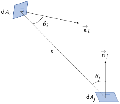
Calculation of View Factor

In the S2S modelling equation 5.426, the view factor, is the proportion of the radiation which leaves surface “" and strikes surface “". As shown in Figure 5.168, assuming that and are the differential areas on the surface “" and “", respectively, and the distance between them is , we can express the view factor from to at a distance as follows:

5.429

where and are the angle between the surface normal directions and a ray between the two differential areas.

Figure 5.168 - Two Differential Areas in an Arbitrary Configuration

If and are the given areas of surface “" and “", respectively, the view factor from surface “" to surface “" is the area averaged integral of equation 5.429 over the surfaces “" and “":

5.430

Note that the surface-to-surface radiation can only occur when the two surfaces are visible to each other, or the view factor is non-zero. Introducing the Kronecker symbol with respect to the visibility between and :

5.431

We can rewrite equation 5.430 as:

5.432

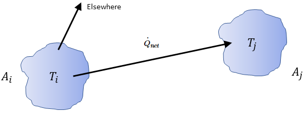
In general, for any two surfaces visible to each other, a given surface “" only radiates a portion of the outgoing radiative energy to the surface “", as shown in Figure 5.169. Therefore, the dimensionless view factor represents the portion of energy that leaves surface “" and reaches surface “". It has the following characteristics:

Figure 5.169 - Radiation between two arbitrary surfaces

Summation of View Factors

Since radiation leaving a surface is conserved, the sum of all view factors from a given surface “" is unity. For an -surface enclosed system, we have

5.433

Self-Viewing Surfaces

Since radiation travels in straight lines, no radiation ray from a convex surface can leave the surface and then hit the same surface later. Hence, the convex surfaces cannot be self-viewed:

5.434

For concave surfaces, the outgoing ray from one position on the surface may hit the same surface later at a different position. Therefore, the concave surface can be visible to itself:

5.435

Superposition

In an -surface system, if a given surface “" radiates to -number of surfaces (), the view factor between the surface “" and the -number of surfaces equals to the sum of the view factors between surface “" and each one of the -number of surfaces:

5.436

The so-called superposition rule (or summation rule) is useful when some geometry is not available with given charts or graphs. The superposition rule allows one to express the geometry that is being sought using the sum or difference of geometries that are known.

Reciprocity

equation 5.432 gives the view factor , defined as the fraction of the radiative energy that leaves the surface “" and reaches surface “". Similarly, the view factor (the portion of energy that leaves the surface “" and reaches surface “") can be expressed as:

5.437

By comparing equation 5.437 with equation 5.432, one can easily obtain the following relationship:

5.438

equation 5.438 is commonly referred to as the reciprocity of the view factors. This reciprocity theorem allows one to directly calculate only one of the pair of view factors.

Clustering

The S2S radiation model can be computationally very expensive when the number of radiating surfaces becomes very large. To reduce both the computational time and the storage requirement, the number of radiating surfaces can be reduced by grouping a certain number of the neighboring boundary-cell faces to create surface "clusters". The radiosity () is then calculated for surface clusters. These values are then distributed to the boundary-cell faces within each cluster to calculate the wall temperatures. Since the radiation source terms are highly non-linear (proportional to the fourth power of temperature), care must be taken to calculate the average temperature of the surface clusters and distribute the flux and source terms appropriately among the boundary faces forming the clusters.

The surface cluster temperature is obtained by area-averaging of boundary face temperature as shown in the following equation:

5.439

where is the temperature of the surface cluster, and and are the face area and temperature of the boundary cell in CFD simulations. The summation is carried over all the faces within a surface cluster.