Boundary Conditions
|
The boundary condition parameters for the Flow module apply to Boundaries. They also apply to Interfaces for which the Flow module is Blanked on one side of the interface, creating in effect, a boundary. The boundary conditions and associated Flow parameters are specified as follows: The equations for the boundary conditions are explained in Modelling of Flow Boundaries. The boundary conditions available for Flow module are: |
Figure 5.25 - Flow Boundary Condition |
Wall
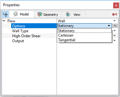
This corresponds to a solid boundary and means that there is shear (drag) and no normal component of velocity at the boundary (i.e. no through-flow). When the Turbulence module is active, the roughness of the wall can be accounted for using Wall Roughness Model. A Wall boundary can be assigned a shear wall velocity using Options.
Options
|
To introduce shear at the wall, the Wall boundary condition has the following Options:
The velocity for a Wall boundary is intended to introduce a shear at the wall. In this case, only tangential velocities are used. Numerically, the velocity for a Wall boundary introduces a momentum source into the momentum equation 5.13. It does not actually move the boundary, i.e. it does not change the shape of the domain. |
Figure 5.26 - Flow Options |
 components of velocity. The velocity at a
 Wall Type
-
Rigid: Produces a non-deforming wall.
- Flexible: Produces a deforming wall. It does not physically move the grid associated with the wall. The effect of the wall motion is included by changing the effective volume of the neighboring cell.

Figure 5.27 - Flow Wall Type
To model flexible walls, there are two models under Deformation Model:
- Elastic Pipe Model: Requires Radius, Wall Thickness, Young’s Modulus, Poisson Ratio, and Reference Pressure as inputs.
- User Defined: Specify the Displacement as a function of pressure using an analytical expression or in table format.
The Displacement and Wall Velocity on the flexible wall can be displayed through the variable list under the Results Panel. These are not reflected in the X-Y Plots.
High Order Shear
This uses a parabolic function for the velocity profile near the wall instead of a linear function. This can be used for laminar flow near the wall. This can also be used if the near wall cell is within the laminar sub-layer for turbulent flows. This reduces the number of cells used to resolve the flow within thin gaps, which are heavily dominated by viscous shear forces.

Figure 5.28 - Flow High Order Shear
Specified Velocity
This sets the velocity on the boundary. The net mass flow out of the boundary is given by the fluid density and velocity (relative to the boundary area and orientation). Choose one of the following to specify the direction and magnitude of the velocity.
 velocity components relative to the model coordinate system.
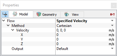
|
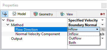
Note: For either Inflow or Outflow, a negative Normal Velocity Component will be reset to a positive value, such that the sign of the Value for the Volumetric Flux has no influence on the direction of flow. |
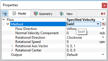
Swirl: This defines a swirling flow at a boundary. The magnitude of the inflow is controlled by the Normal Velocity Component. The Flow Direction can be Inflow , Outflow or Both. The Swirl velocity is given through the: Rotational Direction, Rotational Speed, Rotational Center and Rotational Axis Vector |
Figure 5.31 - Specified Velocity - Swirl |
Specified Volumetric Flux
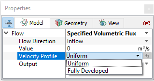
This sets the fluid’s volumetric flux (m3/s) at an opening. Thereby, it sets the velocity at the boundary. The corresponding mass flow is determined by the fluid density and velocity (relative to the boundary area and orientation). The velocity associated can be either Uniform or Fully Developed. The direction and magnitude of the velocity can be specified by the following options:
|
Figure 5.32 - Specified Volumetric Flux - Flow Direction |
||
|
Figure 5.33 - Specified Volumetric Flux - Velocity Profile |
 is input under
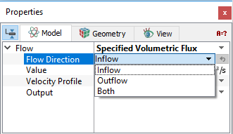
 , boundary area
  and orientation:
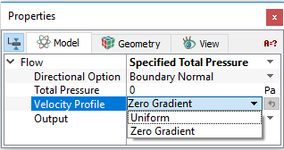
Specified Total Pressure
This defines the total pressure at an opening where flow is expected to enter or leave the domain. The velocity of the flow at the boundary is then computed as part of the solution.
The direction of the boundary velocity vector is given as Cartesian and Boundary Normal under the drop down list of Directional Option.
|
Velocity Profile: The following two options are available:
|
Figure 5.34 - Specified Total Pressure - Velocity Profile |
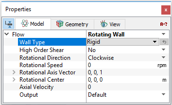
Rotating Wall
This simulates the shear effect of a rotating wall. It requires specifying the following:
|
Figure 5.35 - Rotating Wall |
Symmetry
This means that there is no shear (i.e. perfect slip) and no normal component of velocity at the boundary (i.e. no through-flow). Symmetry for flow also means there is no normal gradient of pressure at the boundary. This boundary condition is different from a wall boundary condition in that for a wall there is shear. This usually corresponds to a physical symmetry in the model, but it doesn’t have to as long as the effects of this boundary condition make sense. For example, it can be used in some cases to mimic a free surface.
Specified Pressure Outlet
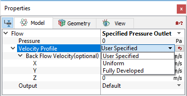
This allows to set the static pressure at an opening where flow is expected to exit the domain. In case of back flow, a momentum source may also be added via the associated Back Flow Velocity (optional)  input. Specified Pressure Outlet determines the mass flow across the boundary as part of the solution.
It has the following options:
-
Pressure: The pressure parameter associated with the Specified Pressure Outlet dictates the static pressure at the outlet. If the properties of the fluid depend on the pressure, pressure should be the absolute pressure, otherwise, it can be a relative pressure (e.g. gauge).
- Velocity Profile: This may be set to the following:
-
Uniform: Allows the velocity at the outlet to be uniform.
- Fully Developed: Allows the velocity profile at the boundary to be similar (same shape) to the velocity profile at the cell centers immediately downstream.
- User Specified: The Back Flow Velocity (optional) parameter associated with the Specified Pressure Outlet allows the user to include a momentum source for any back flow at this boundary. The values are input in terms of the
 components of the velocity. The Back Flow Velocity (optional) does not directly affect the mass flow, it just adds (or subtracts) momentum sources to any fluid flowing back into the domain. Flow can enter or exit the domain at this boundary condition. If flow exits the domain here, the value of the Back Flow Velocity (optional) has no effect. It can be important if the incoming fluid has a relatively high dynamic head.
|
|
Figure 5.36 - Specified Pressure Outlet - Velocity Profile |
Specified Pressure Inlet
This allows to set the static pressure at an opening where flow is expected to enter the domain. A momentum source may also be added at this type boundary via the associated velocity input. Specified Pressure Inlet determines the mass flow across the boundary as part of the solution.
It has following options:
-
Pressure: The pressure parameter associated with the Specified Pressure Inlet dictates the static pressure at the inlet. The effects of the dynamic pressure may be included using the optional velocity (Optional). If the incoming fluid has a relatively high dynamic head, another option is to use the Specified Total Pressure boundary condition instead of Specified Pressure Inlet.
-
Velocity Profile: This may be set to the following:
-
Uniform: Allows the velocity at the inlet to be uniform.
- Fully Developed: Allows the velocity profile at the boundary to be similar (same shape) to the velocity profile at the cell centers immediately downstream.
- User Specified: A back flow velocity can be specified. The Velocity (optional) parameter associated with the Specified Pressure Inlet allows the user to include a momentum source for inflow at this boundary. The values are input in terms of the
 components of the velocity. Velocity (optional) does not directly affect the mass flow, it just adds (or subtracts) momentum sources to the entering fluid. Flow can enter or exit the domain at a Specified Pressure Inlet boundary. If flow exits the domain at a Specified Pressure Inlet, the values of the Velocity (optional) have no effect. It can be important if the incoming fluid has a relatively high dynamic head.
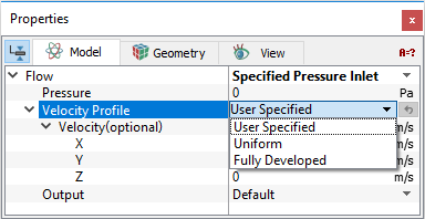
Figure 5.37 - Specified Pressure Inlet - Velocity Profile
-
|
Note: If the incoming fluid has a relatively high dynamic head, another option is to use the Specified Total Pressure boundary condition instead of Specified Pressure Inlet. |
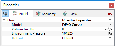
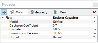
Resistor Capacitor
Resistor Capacitor: This enables the user to determine the flow ( ) - pressure (
 ) relationship for a selected boundary. The following models are available under Model option.
|
Figure 5.38 - Resistor capacitor - DP-Q Curve |
|
|
Figure 5.39 - Resistor Capacitor - Orifice |
|
|
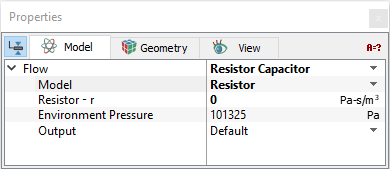
Figure 5.40 - Resistor Capacitor - Resistor |
|
|
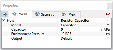
Figure 5.41 - Resistor Capacitor - Capacitor |
|
|
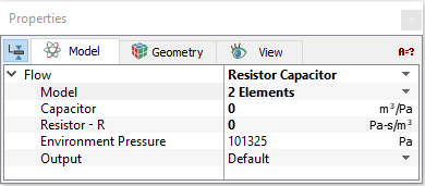
Figure 5.42 - Resistor Capacitor - 2 Elements |
|
|
Figure 5.43 - Resistor Capacitor - Orifice |
 .
.
|
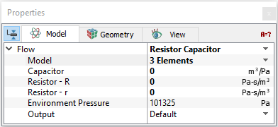
Note: This boundary condition is based on the 2-element and 3-element Windkessel model1 Daniel R. Kerner, Ph.D. . and Broemser, Ph., et. al., ``Uber die Messung des Schlagvolumens des Herzens auf unblutigem Weg'', Zeitung für Biologie 90 (1930) 467-507. often used for heart flow modelling. |
Interface Condition
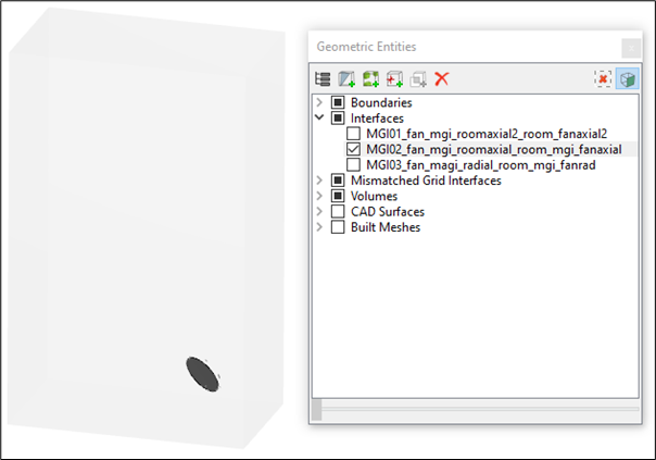
The following interface conditions and associated Flow parameters can be specified for a selected Interface.
Default Interface is the default option for an interface connecting fluid to fluid. The Interface Conditions for the Flow module are the same as for the boundary conditions, if and only if one side of the Interface has been Blanked for Flow. If, instead, the Flow module is Active on both sides of an Interface, then it can only be assigned as a Default Interface. The interfaces can be modelled as:
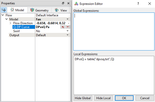
- Fan: Requires specifying the Flow Direction, DP-Q Curve for flow-pressure relationship and Swirl(specified using Center, Tangential Velocity and Radial Velocity). Refer Example of adding Fan curve.
- Pressure Jump: Requires specifying the Flow Direction, DP-Q Curve for flow-pressure relationship and Swirl(specified using Center, Tangential Velocity and Radial Velocity). Refer Example of adding Fan curve.
- Porous Surface: Enables the addition of a resistance due to a permeable interface connecting fluid to fluid. The variables associated with the Surface Porous model are: Thickness, Permeability and Quadratic Coefficient. The pressure drop per unit distance across the interface is computed using the Darcy's Law. The pressure drop across the Interface is computed by multiplying F by some finite thickness. The Porosity is set in the Common module. For more information on derivation of porous media parameters, refer porous media.
In some applications, user need to add a fan curve when user do not want to model the actual fan geometry or if the geometry is complex. Simerics-MP provides an option to add the fan curves as a condition for an interface using the Expression Editor.
The user can add the fan curve by the following steps:
|
|
Note: For more information on how to add Pressure vs Flow curve in table format, refer Tables in the Expression Editor. |
The Flow module outputs available with the Default Interface include Area, Normal, Mass Flow Rate, Volumetric Flow Rate, Momentum, Pressure Force, Average Total Pressure, Pressure, and Average Static Pressure.