You are here: Physics Modules > Multiphase > Output Variables

5.5.5 Output Variables

This section explains the outputs that are obtained from the Multiphase module. They are categorized as follows:

• Primary Variables
• Property Variables
• Integrated Quantities
• Cycle Avg. Volume Fraction Distribution

 

Note: In order to display the contours and X-Y plots, or to write the outputs into an ascii file, the outputs on each Geometric entity (such as Boundary, Volume, Interface or Points) need to be activated in the Model Tab of the Properties Panel.

 

Primary Variables

Primary Variables are the fundamental variables that characterize the physical process in the module. They are usually obtained by directly solving transport equations or through physical constitutions. The primary variables can be displayed in the GUI Viewing Window for selected Geometric Entities as well as written to the ascii file Filename_points.txt. They can also be viewed as X-Y Plots for Point Probes.

For the Multiphase module, a list of Primary Variables is shown in the table below:

Primary Variables are automatically activated for selected Geometric Entities, including Boundaries, Derived Surfaces, Interfaces, Streamline, Particles and/or Volumes, depending on the modules selected.

 

Property Variables

Property Variables are the physical properties for the fluid(s) and solid(s) in the domain. They are required as a part of the solution. They may be displayed in the GUI Viewing Window for selected Geometric Entities as well as written to the ascii file Filename_points.txt (when activated). They can also be viewed as X-Y Plots for Point Probes.

The components in the Multiphase module assume the same GUI Label and points.txt Label as their parent property, with the component name appended. For example, the label for Mixture Density in the point.txt file is rho as per the parent Flow module. For a component of the mixture it is rho_component_name, e.g. rho_water.

For the Multiphase module, a list of Property Variables is shown in the table below:

As shown in Figure 5.113, Property Variables are automatically activated for output on selected Geometric Entities, including Boundaries, Derived Surfaces, Interfaces, Streamline, Particles and/or Volumes, depending on the modules selected. For Point Probes, however, explicit activation is required. The X-Y plots as shown in Figure 5.114 and Figure 5.115 respectively.

Figure 5.113 - Output activation for Points-Property Variables

Figure 5.114 - Multiphase property variables-GUI Viewing window

Figure 5.115 - Multiphase property variables-Plots

 

Integrated Quantities

An Integrated Output is the averaged or total value of a variable over a Boundary, Interface or Volume. When available and activated, the integrated quantities can be stored in the ascii file Filename_integrals.txt as well as be displayed in the GUI using X-Y Plots.

To access the variables listed below using expressions, the syntax given under Expressions column in Table 5.28 is used with a suffix “@boundary or volume name” such as massfrac_oil = phasecomp.oil.mfa@pipe.

A table of the Integrated Quantities for the Multiphase module is shown below:

For a selected Geometric entity, the integrated outputs must be explicitly activated as shown in Figure 5.116.

 

 

 

 

Figure 5.116 - Output activation-Integrated quantities

 

Cycle Average Volume Fraction Distribution

The Cycle Avg. Volume Fraction Distributionoutput is a spatial distribution of "Time Average" value of volume fraction of a component on Wall or Rotating Wall boundaries. It is the average values during a "Period" of time:

The "Period" is defined as number of time steps of a transient simulation. This “Period” is specified by the Cycle Computation Interval. The Cycle Pressure Distribution output is activated for a selected boundary as follows:

• Click Common in the Model Panel.
• In Properties Panel > Model Tab, set Cycle Computation Interval, which is the number of time steps for the "Period" user wants to calculate time average.
• Select Geometric Entities Panel > Boundaries > [Desired Boundary].
• Select Properties Panel > Model Tab > Multiphase > Component > Output > User Select > Cycle Avg. Volume Fraction Distribution > Yes.

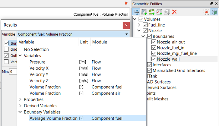
The added outputs are shown in the Results Panel under Variable > Boundary Variablesas shown in Figure 5.118. They are plotted as contours on the selected boundary. The Cycle Avg. Volume Fraction Distribution output is available for Wall and Rotating Wall Boundaries.

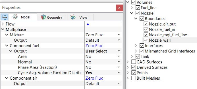
Figure 5.117 - Cycle Avg. Volume Fraction Distribution Boundary condition

Figure 5.118 - Results Display

Note: Cycle Avg. Volume Fraction Distribution is available as output for Wall and Rotating Wall and other solid boundaries (such as as Conjugate Wall Interfaces). Cycle Avg. Volume Fraction Distribution is available as output for the Multiphase Mixture boundaries Zero Flux and Specified Volumetric Flux. Users are recommended to turn on the time average/maximum/minimum output at the very beginning of simulation for all the variables of interest, and use the physical period (i.e. time step for one Pump pocket rotation or a complete revolution) as the “Period” whenever possible.