14.2 Numerics
Numerics pertains to parameters and models used to control the numerical solver to discretize and solve the system of algebraic equations.
- Select the module in the Model Panel.
- Numerics related settings are accessed in the Properties Panel.
When a template is used, the template should be under Extended Mode to access the numerics for the simulation.
Time Accuracy
|
Time accuracy methods offer the following three temporal discretization schemes for solving the variables implicitly.
|
Figure 14.3 - Time accuracy |
 and
and  and
and 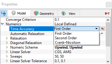
Automatic Relaxation
When selected as Yes in Properties Panel > Model Tab, it adds linear relaxation automatically for the solution of the variable based on mesh quality as shown in equation 14.53.
Relaxation
Controls the amount of correction applied during each iteration, as shown in equation 14.34 and equation 14.53.
- Relaxation range from 0 to 1 whereas typical values of Relaxation range from 0.0 to 0.8.
-
A Relaxation of 0 is the most liberal, allowing full application of the correction. It is recommended, assuming no problem with the convergence. Higher values (>0) are recommended if needed, to prevent the solution from diverging.
-
A Relaxation value of 1 is the most restrictive, allowing no correction of the solution from one iteration to the next.
| Note: For Pressure, there is also an Automatic Relaxation. |
Diagonal Relaxation
Diagonal Relaxation is a form of relaxation applied to the diagonal of the solution matrix as shown in equation 14.25. It has an effect similar to the influence of an old value at a previous time-step. During the solution process, the solver provides an estimate of the amount of correction needed to obtain an accurate solution. In general, Relaxation refers to the amount of this suggested correction that is applied for the next iteration. For the Flow module, there are separate values for the velocity and pressure corrections.
-
Diagonal Relaxation range from 0 to infinity, however typical values of Diagonal Relaxation range from 0.001 to 1.
-
Default values are recommended, assuming no problem with the convergence. Higher values (> 0.3) are recommended if needed to prevent a solution from diverging.
-
A Diagonal Relaxation of 0 is the most liberal, allowing full application of the correction.
- A large value of Diagonal Relaxation is the most conservative, slowing down the corrections from one iteration to the next.
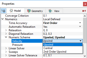
Numeric Scheme
|
Numeric Scheme offers the following three spatial interpolation schemes for solving the variables.
|
Figure 14.4 - Numerics scheme |
|
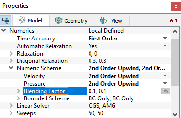
The Blending Factor and the Bounded Scheme are used to stabilize convergence. Blending FactorBlending Factor is used in conjunction with the higher order interpolation schemes (e.g. Central and 2nd Order Upwind) to help stabilize the convergence.
Bounded SchemeBounded Scheme is used in conjunction with the higher order interpolation schemes (e.g. Central and 2nd Order Upwind) to help stabilize the convergence by limiting the range of the value of the interpolation to be no more or less than the maximum or minimum (respectively) of the cells neighboring the cell-face of interest.
A Bounded Scheme can be set for either Central or 2nd Order Upwind in the Properties Panel. There are three options:
|
Figure 14.5 - 2nd order upwind |

Linear Solver Tolerance
The solution process in Simerics-MP is iterative, including for the linear solvers. The user can control the iterative process for any module by setting the Linear Solver Tolerance to the desired convergence tolerance under:
Properties Panel > Model Tab > Numerics > Linear Solver Tolerance > Desired Values.
-
Linear Solver Tolerance dictates the linear solver convergence criterion for solutions of the variables.
-
A smaller value of Linear Solver Tolerance implies more precision.
-
The cost of a smaller value of Linear Solver Tolerance is more sweeps, resulting in more computation time. In some cases, the added accuracy is not worth the additional expense. If the target converge criterion is too small, the solver may not be able to achieve it, in which case the solution will go the full number of sweeps allowed.
The tolerance is normalized relative to the first iteration at the start of the time-step or a steady-state simulation.
Sweeps
The solution process in Simerics-MP is iterative, including the linear solver. The user can control the iterative process for any module by setting the sweeps to a maximum allowed value under:
Properties Panel > Model Tab > Numerics > Sweeps > Desired Values.
- If the solver reaches the maximum sweeps, it will advance to the next variable. The default number for Sweeps is 50 for both the pressure and velocity solvers.
- Number of sweeps is also controlled by the Linear Solver Tolerance. In general the solver should attain the desired tolerance before hitting the maximum number of sweeps.
The number of sweeps used for a given iteration are displayed in the *.out file as follows:
INFO(Sim02:Flow:V:CGS): Residual: 4.19235 Sweeps = 1
INFO(Sim02:Flow:P:AMG): Residual: 52.4886 Sweeps = 2
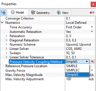
Pressure Velocity Coupling MethodSimerics-MP offers the following three Pressure Velocity Coupling Methods for coupling the pressure and velocity and solutions.
The default Pressure Velocity Coupling Method for Simerics-MP is SimpleS. |
Figure 14.7 - Pressure Velocity Coupling |
Skew Term
Skew Terms in the Turbulence module for Turbulent Kinetic Energy (TKE) and the Turbulent Energy Dissipation Rate (TEDR) solution can be activated as follows:
Model Panel > Turbulence
Properties Panel > Model Tab > Numerics > Skew Term > [Yes or No]
Skew Terms refer to the links between diagonally connected cells in the mesh. These terms typically offer negligible improvement in the solution, while potentially slowing down the calculation. By default they are not used in the solution of the Turbulence module.
Max. Temperature Adjustment
The Max. Temperature Adjustment in the Heat module is accessed as follows:
Model Panel > Heat
Properties Panel > Model Tab > Numerics > Max. Temperature Adjustment > [Desired Value]
This limits the amount the temperature may vary during the predictor-corrector solution process. The Max. Temperature Adjustment is used to stabilize convergence similar to a Relaxation Factor. A smaller value of Max. Temperature Adjustment is more stable and could use more computer time.
Temperature Lower Limit
The temperature throughout the solution domain can be constrained to be at or above the Temperature Lower Limit. This can be set in the Heat module as follows:
Model Panel > Heat
Properties Panel > Model Tab > Numerics > Temperature Lower Limit > [Desired Value]
The default value for the Temperature Lower Limit is 0.1 K. and is very close to Absolute Zero. It is possible to set the Temperature Lower Limit less than 0 and to solve for negative temperatures in Simerics. In such cases, the absolute temperature scale becomes meaningless and unphysical results would result if the “temperature” were being used to determine physical properties. The setting of a Temperature Lower Limit is a constraint intended to help convergence by bounding the solution during the iterative solution process. If the final solution has temperatures equal to the Temperature Lower Limit, then the solution is over-constrained and the results are most likely unphysical.
Temperature Upper Limit
The temperature throughout the solution domain can be constrained to be at or above the Temperature Upper Limit. This can be set in the Heat module as follows:
Model Panel > Heat
Properties Panel > Model Tab > Numerics > Temperature Upper Limit > [Desired Value]
The default value for the Temperature Upper Limit is 6,000 K. This is greater than the temperature of the surface of the sun, so it is higher than what would typically be encountered in most applications. The setting of a Temperature Upper Limit is a constraint intended to help convergence by bounding the solution during the iterative solution process. If the final solution has temperatures equal to the Temperature Upper Limit, then the solution is over-constrained and the results are most likely unphysical.
Implicit and Explicit methods
This can be accessed as follows:
Model Panel > Multiphase
Properties Panel > Model Tab > Implicit Method > [Yes or No]
- Yes: Solves the Multiphase transport equations implicitly. This method can use larger time-steps than the explicit method but does not preserve the shape of the interface between components as accurately. This updates the transport of a component from one cell to the next based on the most recent iteration estimated volume fraction in each. The implicit method is the solution method used for other scalars (e.g. Heat, Pressure, Multiphase, etc.) and has similar numerical options as explained above and as shown in Figure 14.12.
- No: Solves the Multiphase transport equations explicitly. The explicit method is more accurate than the implicit method in preserving the shape of the interface between components, but it does not work when energy equation is turned-on. This method updates the transport of a component from one cell to the next based on the volume fractions from the previous time-step.
Maximum Courant Number
The Courant Number ( ) in three dimensions is:

|
where  are the components of velocity and
  are the localized dimensions of the mesh cell in the
  directions respectively, and
  is the time-step. For the explicit method, the Courant Number is limited to a value less than 1 to avoid numerical instability.
The sub-time-step ( ) is used in the calculation of the transport of the components for the Multiphase module and is computed based on the courant number.
The calculation of  is performed only for the cells in the domain that have a mixture of components, and then the smallest of those calculations is used as the
  for updating the transport of the components.
This can be accessed as follows:
Model Panel > Multiphase
Properties Panel > Model Tab > Maximum Courant Number
For a transient simulation, if the sub-time-step ( ) computed based on the Courant number is larger than the global time-step set via the Simulation Panel, the smaller of the two is used in the calculation of the transport of the components.
14.2.1 Flow
Numerics under the Flow module are accessed as follows:
Model Panel > Flow
Properties Panel > Model Tab > Numerics > [Local Defined]
The Numerics may be set separately for the pressure and velocity solutions.

Figure 14.8 - Flow numerics parameters
| Flow Module Numerics Options | Default Values/Scheme | Comments | ||
|---|---|---|---|---|
| Time Accuracy | First Order | |||
| Automatic Relaxation | Yes | For Pressure | ||
| Relaxation | 0,0 | Typical values of Relaxation range from 0.0 to 0.8. | ||
|
0 | |||
|
0 | |||
| Diagonal Relaxation | 0.3, 0.3 | There are separate values for the Velocity and Pressure corrections as shown in equation 14.1 and equation 14.1 respectively. | ||
|
0.3 | |||
|
0.3 | |||
| Numeric Scheme | Upwind,Upwind | |||
|
Upwind | |||
|
Upwind | |||
|
0.1, 0.1 | If the Numeric Scheme is set to Central or 2nd Order Upwind for Velocity and Pressure | ||
|
0.1 | |||
|
0.1 | |||
|
BC Only, BC Only | If the Numeric Scheme is set to Central or 2nd Order Upwind for Velocity and Pressure | ||
|
BC Only | |||
|
BC Only | |||
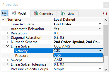
| Linear Solver | CGS, AMG | |||
|
CGS | |||
|
AMG | |||
| Sweeps | 50, 50 |
The number of Sweeps used for a given iteration are displayed in the .out file as follows:
|
||
|
50 | |||
|
50 | |||
| Linear Solver Tolerance | 0.1, 0.1 |
The Residuals for Velocity and Pressure are displayed in the .out file as follows:
|
||
|
0.1 | |||
|
0.1 | |||
| Pressure Velocity Coupling | SimpleS |
14.2.2 Cavitation
For the Cavitation module, the Numerics are set based on the cavitation model used. They are accessed as follows:
Model Panel > Cavitation
Properties Panel > Model Tab > Numerics> [Local Defined]
The parameters available under Numerics for the Cavitation module are shown in .

Figure 14.9 - Cavitation numerics parameters
| Cavitation Module Numerics Options | Default Values/Scheme | Comments | ||
|---|---|---|---|---|
| Time Accuracy | First Order | |||
| Relaxation | 0,0,0 | It is available for all cavitation models. | ||
|
0 | |||
|
0 | |||
|
0 | |||
| Diagonal Relaxation | 0.2, 0.2, 0.2 | It is available for all cavitation models. | ||
|
0.2 | |||
|
0.2 | |||
|
0.2 | |||
| Numeric Scheme | Upwind, Upwind, Upwind | Numeric Scheme may be set separately for the Gas Volume Fraction, Vapor Volume Fraction, and/or Dissolved Gas Volume Fraction models. Blending Factor and Bounded Scheme settings are similar to Flow module. | ||
|
Upwind | |||
|
Upwind | |||
|
Upwind | |||
| Linear Solver | CGS, CGS, CGS | |||
|
CGS | |||
|
CGS | |||
|
CGS |
|||
| Sweeps | 500, 500, 500 |
The number of Sweeps used for a given iteration are displayed in the *.out file as follows:
|
||
|
500 | |||
|
500 | |||
|
500 | |||
| Linear Solver Tolerance | 0.1, 0.1, 0.1 |
The Residuals are displayed in the *.out file as follows:
|
||
|
0.1 | |||
|
0.1 | |||
|
0.1 |
Table 14.2 - Cavitation numerics
The Numerics settings available for the different cavitation models are shown in the Table 14.3.
| Gas Mass Fraction | Vapor Mass Fraction | Dissolved Gas Mass Fraction | |
|---|---|---|---|
| Constant Gas Mass Fraction | Yes | ||
| Equilibrium Dissolved Gas Model | Yes | ||
| Variable Gas Mass Fraction | Yes | Yes | |
| Dissolved Gas Model | Yes | Yes | |
| Full Gas Model | Yes | Yes | Yes |
14.2.3 Turbulence
Numerics under the Turbulence module are accessed as follows:
Model Panel > Turbulence
Properties Panel > Model Tab > Numerics> [Local Defined]
The Numerics may be set separately for the Turbulent Kinetic Energy and the Turbulent Energy Dissipation Rate solutions.

Figure 14.10 - Turbulence numerics parameters
| Turbulence Module Numerics Options | Default Values/Scheme | Comments | ||
|---|---|---|---|---|
| Time Accuracy | First Order | |||
| Relaxation | 0,0 | |||
|
0 | |||
|
0 | |||
| Diagonal Relaxation | 0.3, 0.3 | |||
|
0.3 | |||
|
0.3 | |||
| Numeric Scheme | Upwind,Upwind | Blending Factor and Bounded Scheme settings are similar to Flow module. | ||
|
Upwind | |||
|
Upwind | |||
| Linear Solver | CGS, CGS | |||
|
CGS | |||
|
CGS |
|||
| Sweeps | 500, 500 |
The number of Sweeps used for a given iteration are displayed in the *.out file as follows:
|
||
|
500 | |||
|
500 | |||
| Linear Solver Tolerance | 0.1, 0.1 |
The Residuals for Turbulent Kinetic Energy and the Turbulent Energy Dissipation Rate are displayed in the *.out file as follows:
|
||
|
0.1 | |||
|
0.1 | |||
| Skew Term | No |
Table 14.4 - Turbulence numerics
14.2.4 Heat
Numerics under the Heat module to control the solver for the energy equation (enthalpy) are accessed as follows:
Model Panel > Heat
Properties Panel > Model Tab > Numerics> [Local Defined]

Figure 14.11 - Heat numerics parameters
| Heat Module Numerics Options | Default Values/Scheme | Comments |
|---|---|---|
| Time Accuracy | First Order | |
| Relaxation | 0 | |
| Diagonal Relaxation | 0 | |
| Numeric Scheme | Upwind | Numerical Schemes for the Heat Module apply to the fluid phase only. In the solid phase, the Central option is used exclusively by default. If central option is selected, then the default values for Blending Factor and Bounded Schemeare 0.1 and BC Only respectively. The same default values apply to 2nd Order Upwindscheme. |
| Linear Solver | AMG | |
| Sweeps | 50 |
The number of Sweeps used for a given iteration are displayed in the *.out file as follows:
|
| Linear Solver Tolerance | 0.1 |
The Residuals for the Heat Module are displayed in the *.out file as follows:
|
| Temperature Upper Limit | 6000 | |
| Temperature Lower Limit | 0.1 | |
| Max. Temperature Adjustment | 5 |
Table 14.5 - Heat numerics
14.2.5 Multiphase
Numerics under the Multiphase module are accessed as follows:
Model Panel > Multiphase
Properties Panel > Model Tab > Numerics > [Local Defined]

| Multiphase Module Numerics Options | Default Values/Scheme | Comments | ||
|---|---|---|---|---|
| Implicit Method | Yes | |||
| Time Accuracy | First Order | |||
| Relaxation | 0.5 | |||
| Diagonal Relaxation | 0.5 | |||
| Numeric Scheme | High Resolution | Blending Factor and Bounded Scheme settings are similar to Flow module. | ||
|
0 | |||
|
1 | |||
| Linear Solver | CGS | |||
| Sweeps | 500 |
The number of Sweeps used for a given iteration are displayed in the *.out file as follows:
|
||
| Linear Solver Tolerance | 0.1 |
|
||
| Maximum Courant Number | 5 |
Table 14.6 - Multiphase numerics
14.2.6 Multicomponent
Numerics under the Multicomponent Mixing module are accessed as follows:
Model Panel > Heat > Multicomponent Mixing
Properties Panel > Model Tab > Numerics > [Local Defined]

Figure 14.13 - Multicomponent mixing numerics parameters
| Multicomponent Mixing Module Numerics Options | Default Values/Schemes | Comments |
|---|---|---|
| Time Accuracy | First Order | |
| Relaxation | 0 | |
| Diagonal Relaxation | 0 | |
| Numeric Scheme | Upwind | |
| Linear Solver | AMG | |
| Sweeps | 50 |
The number of Sweeps used for a given iteration are displayed in the *.out file as follows:
|
| Linear Solver Tolerance | 0.1 |
Table 14.7 - Multicomponent mixing numerics
14.2.7 Species
Numerics under the Species module are accessed as follows:
Model Panel > Species [Name]
Properties Panel > Model Tab > Numerics > [Local Defined]

Figure 14.14 - Species numerics parameters
| Species Module Numerics Options | Default Values/Schemes | Comments |
|---|---|---|
| Time Accuracy | First Order | |
| Relaxation | 0 | |
| Diagonal Relaxation | 0.3 | |
| Numeric Scheme | Upwind | |
| Linear Solver | AMG | |
| Sweeps |
50 |
The number of Sweeps used for a given iteration are displayed in the *.out file as follows
|
| Linear Solver Tolerance | 0.1 |
Table 14.8 - Species numerics